5: Testing Hypotheses
- Page ID
- 5322
\( \newcommand{\vecs}[1]{\overset { \scriptstyle \rightharpoonup} {\mathbf{#1}} } \)
\( \newcommand{\vecd}[1]{\overset{-\!-\!\rightharpoonup}{\vphantom{a}\smash {#1}}} \)
\( \newcommand{\dsum}{\displaystyle\sum\limits} \)
\( \newcommand{\dint}{\displaystyle\int\limits} \)
\( \newcommand{\dlim}{\displaystyle\lim\limits} \)
\( \newcommand{\id}{\mathrm{id}}\) \( \newcommand{\Span}{\mathrm{span}}\)
( \newcommand{\kernel}{\mathrm{null}\,}\) \( \newcommand{\range}{\mathrm{range}\,}\)
\( \newcommand{\RealPart}{\mathrm{Re}}\) \( \newcommand{\ImaginaryPart}{\mathrm{Im}}\)
\( \newcommand{\Argument}{\mathrm{Arg}}\) \( \newcommand{\norm}[1]{\| #1 \|}\)
\( \newcommand{\inner}[2]{\langle #1, #2 \rangle}\)
\( \newcommand{\Span}{\mathrm{span}}\)
\( \newcommand{\id}{\mathrm{id}}\)
\( \newcommand{\Span}{\mathrm{span}}\)
\( \newcommand{\kernel}{\mathrm{null}\,}\)
\( \newcommand{\range}{\mathrm{range}\,}\)
\( \newcommand{\RealPart}{\mathrm{Re}}\)
\( \newcommand{\ImaginaryPart}{\mathrm{Im}}\)
\( \newcommand{\Argument}{\mathrm{Arg}}\)
\( \newcommand{\norm}[1]{\| #1 \|}\)
\( \newcommand{\inner}[2]{\langle #1, #2 \rangle}\)
\( \newcommand{\Span}{\mathrm{span}}\) \( \newcommand{\AA}{\unicode[.8,0]{x212B}}\)
\( \newcommand{\vectorA}[1]{\vec{#1}} % arrow\)
\( \newcommand{\vectorAt}[1]{\vec{\text{#1}}} % arrow\)
\( \newcommand{\vectorB}[1]{\overset { \scriptstyle \rightharpoonup} {\mathbf{#1}} } \)
\( \newcommand{\vectorC}[1]{\textbf{#1}} \)
\( \newcommand{\vectorD}[1]{\overrightarrow{#1}} \)
\( \newcommand{\vectorDt}[1]{\overrightarrow{\text{#1}}} \)
\( \newcommand{\vectE}[1]{\overset{-\!-\!\rightharpoonup}{\vphantom{a}\smash{\mathbf {#1}}}} \)
\( \newcommand{\vecs}[1]{\overset { \scriptstyle \rightharpoonup} {\mathbf{#1}} } \)
\(\newcommand{\longvect}{\overrightarrow}\)
\( \newcommand{\vecd}[1]{\overset{-\!-\!\rightharpoonup}{\vphantom{a}\smash {#1}}} \)
\(\newcommand{\avec}{\mathbf a}\) \(\newcommand{\bvec}{\mathbf b}\) \(\newcommand{\cvec}{\mathbf c}\) \(\newcommand{\dvec}{\mathbf d}\) \(\newcommand{\dtil}{\widetilde{\mathbf d}}\) \(\newcommand{\evec}{\mathbf e}\) \(\newcommand{\fvec}{\mathbf f}\) \(\newcommand{\nvec}{\mathbf n}\) \(\newcommand{\pvec}{\mathbf p}\) \(\newcommand{\qvec}{\mathbf q}\) \(\newcommand{\svec}{\mathbf s}\) \(\newcommand{\tvec}{\mathbf t}\) \(\newcommand{\uvec}{\mathbf u}\) \(\newcommand{\vvec}{\mathbf v}\) \(\newcommand{\wvec}{\mathbf w}\) \(\newcommand{\xvec}{\mathbf x}\) \(\newcommand{\yvec}{\mathbf y}\) \(\newcommand{\zvec}{\mathbf z}\) \(\newcommand{\rvec}{\mathbf r}\) \(\newcommand{\mvec}{\mathbf m}\) \(\newcommand{\zerovec}{\mathbf 0}\) \(\newcommand{\onevec}{\mathbf 1}\) \(\newcommand{\real}{\mathbb R}\) \(\newcommand{\twovec}[2]{\left[\begin{array}{r}#1 \\ #2 \end{array}\right]}\) \(\newcommand{\ctwovec}[2]{\left[\begin{array}{c}#1 \\ #2 \end{array}\right]}\) \(\newcommand{\threevec}[3]{\left[\begin{array}{r}#1 \\ #2 \\ #3 \end{array}\right]}\) \(\newcommand{\cthreevec}[3]{\left[\begin{array}{c}#1 \\ #2 \\ #3 \end{array}\right]}\) \(\newcommand{\fourvec}[4]{\left[\begin{array}{r}#1 \\ #2 \\ #3 \\ #4 \end{array}\right]}\) \(\newcommand{\cfourvec}[4]{\left[\begin{array}{c}#1 \\ #2 \\ #3 \\ #4 \end{array}\right]}\) \(\newcommand{\fivevec}[5]{\left[\begin{array}{r}#1 \\ #2 \\ #3 \\ #4 \\ #5 \\ \end{array}\right]}\) \(\newcommand{\cfivevec}[5]{\left[\begin{array}{c}#1 \\ #2 \\ #3 \\ #4 \\ #5 \\ \end{array}\right]}\) \(\newcommand{\mattwo}[4]{\left[\begin{array}{rr}#1 \amp #2 \\ #3 \amp #4 \\ \end{array}\right]}\) \(\newcommand{\laspan}[1]{\text{Span}\{#1\}}\) \(\newcommand{\bcal}{\cal B}\) \(\newcommand{\ccal}{\cal C}\) \(\newcommand{\scal}{\cal S}\) \(\newcommand{\wcal}{\cal W}\) \(\newcommand{\ecal}{\cal E}\) \(\newcommand{\coords}[2]{\left\{#1\right\}_{#2}}\) \(\newcommand{\gray}[1]{\color{gray}{#1}}\) \(\newcommand{\lgray}[1]{\color{lightgray}{#1}}\) \(\newcommand{\rank}{\operatorname{rank}}\) \(\newcommand{\row}{\text{Row}}\) \(\newcommand{\col}{\text{Col}}\) \(\renewcommand{\row}{\text{Row}}\) \(\newcommand{\nul}{\text{Nul}}\) \(\newcommand{\var}{\text{Var}}\) \(\newcommand{\corr}{\text{corr}}\) \(\newcommand{\len}[1]{\left|#1\right|}\) \(\newcommand{\bbar}{\overline{\bvec}}\) \(\newcommand{\bhat}{\widehat{\bvec}}\) \(\newcommand{\bperp}{\bvec^\perp}\) \(\newcommand{\xhat}{\widehat{\xvec}}\) \(\newcommand{\vhat}{\widehat{\vvec}}\) \(\newcommand{\uhat}{\widehat{\uvec}}\) \(\newcommand{\what}{\widehat{\wvec}}\) \(\newcommand{\Sighat}{\widehat{\Sigma}}\) \(\newcommand{\lt}{<}\) \(\newcommand{\gt}{>}\) \(\newcommand{\amp}{&}\) \(\definecolor{fillinmathshade}{gray}{0.9}\)Since the beginning of the text it has been emphasized that a primary reason for doing statistics is to make a decision. Better decisions can be made if they are based on the best available evidence. While the ideal situation would be to get data from the entire population, the reality is that data will almost always come from a sample. Because sample data varies based on the random process that was used to select it, the researcher is forced to use sample data to draw a conclusion about the entire population. This is inference. It is using specific partial evidence to make a more general conclusion.
In Chapter 5, formulas were developed for testing hypotheses about proportions and means. In the former case the formula was
\[z = \dfrac{\hat{p} - p}{\dfrac{p(1 - p)}{n}}\]
and in the latter case it was
\[z = \dfrac{\bar{x} - \mu}{\dfrac{\sigma}{\sqrt{n}}}.\]
In general, these formulas generate a test statistic, z, which is used to determine the number of standard errors a statistic is from a parameter. The normal distribution is then used to determine the probability of getting that statistic, or a more extreme statistic. That probability is called a p-value.
Every number that is needed to make use of the formula
\[z = \dfrac{\hat{p} - p}{\dfrac{p(1 - p)}{n}}\]
can be found in the null hypothesis (p) or from the data (\(\hat{p}\), \(n\)). The same cannot be said for the formula
\[z = \dfrac{\bar{x} - \mu}{\dfrac{\sigma}{\sqrt{n}}}.\]
While the value for \(\mu\) comes from the null hypothesis and the value of \(\bar{x}\) and n come from the sample data, there is no way to obtain the value of \(\sigma\) without doing a census. In the last chapter you were always told the value of \(\sigma\), but this does not happen in the real world because to find \(\sigma\) requires first finding \(\mu\) and if you knew \(\mu\), there would be no reason to test a hypothesis about it.
The resolution of this problem requires two changes to the process that was used in the previous chapter. The first change is that we will have to estimate \(\sigma\). The best estimate is s, the standard deviation of the sample. Replacing \(\sigma\) with s means we can no longer use the standard normal distribution (z distribution). The second change therefore is to find a more appropriate distribution that can be used to model the distribution of sample means.
A set of distributions called the t distributions is used when the standard error of the mean, \(\sigma_{\bar{x}} = \dfrac{\sigma}{\sqrt{n}}\) is replaced with the estimated standard error of the mean \(s_{\bar{x}} = \dfrac{s}{\sqrt{n}}\). The z formula for means,
\[z = \dfrac{\bar{x} - \mu}{\dfrac{\sigma}{\sqrt{n}}}\]
is then modified to become the t formula
\[t = \dfrac{\bar{x} - \mu}{\dfrac{s}{\sqrt{n}}}.\]
Notice the only difference is the use of s instead of \(\sigma\). The t distributions are used because they provide a better approximation of the distribution of sample means when the population standard deviation must be estimated using the sample standard deviation.
Unlike the normal distribution, there are many t distributions with each being defined by the number of degrees of freedom. Degrees of Freedom are a new concept that requires a little explanation.
The concept of degrees of freedom has to do with the number of independent values that can identify a position. This may be easier to think about if you picture a Cartesian coordinate system. With any two independently chosen values, normally called x and y, a point’s position can be located somewhere on the graph. Consequently, the point that is picked has two degrees of freedom. However, if a constraint is placed on the points, such as x + y = 3, then only one of the values can be independent and the other value will depend on the independent value. Because of the constraint, one degree of freedom has been lost so now the point has only one degree of freedom. If a second constraint is placed on the system, such as x – y = 1, then another degree of freedom is lost. Degrees of freedom are lost every time a constraint is applied.
For sample data, each value represents a new piece of evidence, provided the data are independent. Dependent data would artificially inflate the sample size without providing any more information. Since a larger sample size would produce a smaller standard error, which would lead to a larger t value and therefore increase the chance of a statistically significant conclusion, then it is important to only count the number of independent data values, which are known as degrees of freedom. One degree of freedom is lost every time a parameter is replaced by a statistic. Therefore, when the standard error \(\sigma_{bar{x}} = \dfrac{\sigma}{\sqrt{n}}\) becomes the estimated standard error \(s_{\bar{x}} = \dfrac{s}{\sqrt{n}}\), one degree of freedom has been lost. In this case, df = n – 1 where df is an abbreviation for degrees of freedom.
The formula for generating the test statistic, t, that is used to determine the number of standard errors a sample mean is from a hypothesized mean is
\[t = \dfrac{\bar{x} - \mu}{\dfrac{s}{\sqrt{n}}}\]
It has n-1 degrees of freedom.
In the same way that z = 1 represents 1 standard deviation above the mean for a normal distribution, \(t = 1\) represents 1 standard deviation above the mean in a t distribution. Once the value of \(t\) has been determined, the p-value can be found by looking in a t table.
Student t distributions
| One Tail Probability | 0.4 | 0.25 | 0.1 | 0.05 | 0.025 | 0.01 | 0.005 | 0.0005 |
| Two Tail Probability | 0.8 | 0.5 | 0.2 | 0.1 | 0.05 | 0.02 | 0.01 | 0.001 |
| Confidence Level | 20% | 50% | 80% | 90% | 95% | 98% | 99% | 99.9% |
| df | ||||||||
| 1 | 0.325 | 1.000 | 3.078 | 6.314 | 12.706 | 31.821 | 63.656 | 636.578 |
| 2 | 0.289 | 0.816 | 1.886 | 2.920 | 4.303 | 6.965 | 9.925 | 31.600 |
| 3 | 0.277 | 0.765 | 1.638 | 2.353 | 3.182 | 4.541 | 5.841 | 12.924 |
| 4 | 0.271 | 0.741 | 1.533 | 2.132 | 2.776 | 3.747 | 4.604 | 8.610 |
| 5 | 0.267 | 0.727 | 1.476 | 2.015 | 2.571 | 3.365 | 4.032 | 6.869 |
| 6 | 0.265 | 0.718 | 1.440 | 1.943 | 2.447 | 3.143 | 3.707 | 5.959 |
| 7 | 0.263 | 0.711 | 1.415 | 1.895 | 2.365 | 2.998 | 3.499 | 5.408 |
| 8 | 0.262 | 0.706 | 1.397 | 1.860 | 2.306 | 2.896 | 3.355 | 5.041 |
| 9 | 0.261 | 0.703 | 1.383 | 1.833 | 2.262 | 2.821 | 3.250 | 4.781 |
| 10 | 0.260 | 0.700 | 1.372 | 1.812 | 2.228 | 2.764 | 3.169 | 4.587 |
| 11 | 0.260 | 0.697 | 1.363 | 1.796 | 2.201 | 2.718 | 3.106 | 4.437 |
| 12 | 0.259 | 0.695 | 1.356 | 1.782 | 2.179 | 2.681 | 3.055 | 4.318 |
| 13 | 0.259 | 0.694 | 1.350 | 1.771 | 2.160 | 2.650 | 3.012 | 4.221 |
| 14 | 0.258 | 0.692 | 1.345 | 1.761 | 2.145 | 2.624 | 2.977 | 4.140 |
| 15 | 0.258 | 0.691 | 1.341 | 1.753 | 2.131 | 2.602 | 2.947 | 4.073 |
| 16 | 0.258 | 0.690 | 1.337 | 1.746 | 2.120 | 2.583 | 2.921 | 4.015 |
| 17 | 0.257 | 0.689 | 1.333 | 1.740 | 2.110 | 2.567 | 2.898 | 3.965 |
| 18 | 0.257 | 0.689 | 1.330 | 1.734 | 2.101 | 2.552 | 2.878 | 3.922 |
| 19 | 0.257 | 0.688 | 1.328 | 1.729 | 2.093 | 2.539 | 2.861 | 3.883 |
| 20 | 0.257 | 0.687 | 1.325 | 1.725 | 2.086 | 2.528 | 2.845 | 3.850 |
| 21 | 0.257 | 0.686 | 1.323 | 1.721 | 2.080 | 2.518 | 2.831 | 3.819 |
| 22 | 0.256 | 0.686 | 1.321 | 1.717 | 2.074 | 2.608 | 2.819 | 3.792 |
| 23 | 0.256 | 0.685 | 1.319 | 1.714 | 2.069 | 2.500 | 2.807 | 3.768 |
| 24 | 0.256 | 0.685 | 1.318 | 1.711 | 2.064 | 2.492 | 2.797 | 3.745 |
| 25 | 0.256 | 0.684 | 1.316 | 1.708 | 2.060 | 2.485 | 2.787 | 3.745 |
| 26 | 0.256 | 0.684 | 1.315 | 1.706 | 2.056 | 2.479 | 2.779 | 3.707 |
| 27 | 0.256 | 0.684 | 1.314 | 1.703 | 2.052 | 2.473 | 2.771 | 3.689 |
| 28 | 0.256 | 0.683 | 1.313 | 1.701 | 2.048 | 2.467 | 2.763 | 3.674 |
| 29 | 0.256 | 0.683 | 1.311 | 1.699 | 2.045 | 2.462 | 2.756 | 3.660 |
| 30 | 0.256 | 0.683 | 1.310 | 1.697 | 2.042 | 2.457 | 2.750 | 3.646 |
| 40 | 0.255 | 0.681 | 1.303 | 1.684 | 2.021 | 2.423 | 2.704 | 3.551 |
| 60 | 0.254 | 0.679 | 1.296 | 1.671 | 2.000 | 2.390 | 2.660 | 3.460 |
| 120 | 0.254 | 0.677 | 1.289 | 1.658 | 1.980 | 2.358 | 2.617 | 3.373 |
| \(z^{\ast}\) | 0.253 | 0.674 | 1.282 | 1.645 | 1.960 | 2.326 | 2.576 | 3.290 |
An assumption when using t distributions with a small sample size is that the sample is drawn from a normally distributed population. While some researchers believe this test statistic is robust enough to tolerate some violation of this assumption, at a minimum, a histogram of the data should be viewed to see if the assumption appears realistic. If it does not, other methods of analysis not discussed in this text must be pursued.
The way this t table is used to determine a p-value is to first find the row with the appropriate number of degrees of freedom. In that row, locate the range that would contain the test statistic. Move up to the first row if you are doing a one-tail test or the second row if it is a two-tail test. Next, identify the location of alpha. If your p-value is greater than alpha then use an inequality symbol to show that. If your p-value is less than alpha then show that with an inequality symbol. If greater detail can be provided, it should be. Since the t distributions are symmetric, negative t values can be found in this table by ignoring the negative signs and assuming the areas in the first row are to the left. Following are 2 examples. The sign in the alternative hypothesis, the level of significance, degrees of freedom, and the t value is provided in each example.
1. \(H_1: > \) \(\alpha = 0.05\) df = 6, t = 2.3

For 6 degrees of freedom, 2.3 falls between 1.943 and 2.447, which means it has an area in the tail that is between 0.05 and 0.025. The p-value would be reported as p < 0.05.
2. \(H_1: \ne \) \(\alpha = 0.01\) df = 18, t = -1.26

For 18 degrees of freedom, -1.26 falls between 0.688 and 1.328 if the negative sign is ignored, so the area in two tails falls between 0.5 and 0.2. Since any value in this range would not be significant at the 0.01 level, then the p-value is greater than 0.01. However, greater detail can be provided by indicating the p-value is greater than 0.2. It would be incorrect to say the p-value is less than 0.5 because that does not tell us whether it is greater or less than 0.01.
There are two different inferential approaches that can be taken. Throughout most of this text the focus has been on the concept of testing hypotheses. That means there is actually a hypothesis of what would be found from a census. The alternative inferential approach occurs when there is not a hypothesis. In such cases the goal is to estimate the parameter rather than determine if the hypothesis about it is correct. Because the entire focus of the book has been on testing hypotheses, we will begin there and then address the idea of estimating the parameter in the next chapter. There are a considerable number of hypothesis test situations and formula, but we will focus on only four of them in this chapter and then add a few more in later chapters. The explanation will be provided with a discussion of exercise.
Briefing 5.1 Exercise
The US government recommends that people get 2.5 hours of moderately-intense aerobic exercise each week or 1.25 hours of vigorous-intense exercise each week along with some strength training such as weights or push-ups. Exercise helps reduce the risk of diabetes, heart disease, some types of cancer and improves mental health. (www.cbsnews.com/8301-204_162-...nded-exercise/)
The four hypothesis-test formulas that will be shown in this chapter will be illustrated with these five questions. As you read the questions, try to determine any similarities or differences between them, as that will ultimately guide you into which formula should be used.
- Is the proportion of people who exercise enough to meet the government’s recommendation less than 0.25?
- Is the proportion of people with a health problem such as diabetes, heart disease or cancer lower for those who meet the government’s exercise recommendation than it is for those who don’t?
- Is the average amount of exercise a college student does in a week greater than 2.5 hours?
- Is the average weight of a person less after a month of new regular aerobic fitness program?
- For those who exercise regularly, is the average amount of exercise a college graduate does in a week different than someone who does not graduate from college?
There are two different things to look for when determining similarities and differences. The first is whether the parameter that is mentioned is a mean or proportion. The second is the number of populations. The following table restates the questions, provides the parameter of interest, the number of populations and an example of the hypotheses.
|
Question |
Parameter |
Populations |
Hypotheses |
|
Is the proportion of people who exercise enough to meet the government’s recommendation less than 0.25? |
proportion |
1 |
\(H_0: P = 0.25\) |
|
Is the proportion of people with a health problem such as diabetes, heart disease or cancer lower for those who meet the government’s exercise recommendation than it is for those who don’t? |
proportion |
2 |
\(H_0: P_{\text{exercise}} = P_{\text{don’t}}\) |
|
Is the average amount of exercise a college student does in a week greater than 2.5 hours? |
mean |
1 |
\(H_0: \mu = 2.5\) |
|
Is the average weight of a person less after a month of new regular aerobic fitness program? |
mean |
1 |
\(H_0: \mu = 0\) |
|
For those who exercise regularly, is the average amount of exercise a college graduate does in a week different than someone who does not graduate from college? |
mean |
2 |
\(H_0: \mu_{\text{college grad}} = \mu_{\text{not college grad}}\) |
Categorical data will be needed for questions about a proportion; quantitative data will be needed for questions about a mean. A brief explanation is needed for the fourth question. To determine the amount of change in a person after starting a fitness program, it is necessary to collect two sets of data. The person will need to be weighed prior to the fitness program and then again after one month. These data are dependent, which means they have to apply to the same person. Ultimately, the data that will be analyzed is the difference between a person’s before and after weight. Therefore two data values are compressed into one value by subtraction. If the after-minus-before difference in weight is 0, then there has been no change. If it is less than 0, weight has been lost.
Since the evidence to help decide which hypothesis is supported by the data will come from a sample, and that sample is just one of the many possible sample results that form a normally distributed sampling distribution, then we can use what is known about the sampling distribution to determine the probability that we would have selected the data we got, or more extreme data (p-value).
In spite of the theoretical nature of a sampling distribution, it is the source for determining probabilities. Therefore, we will first define what the distributions contain and the important formulas related to this distribution.
The first time we encountered the normal distribution was when it was used as an approximation for the binomial distribution. In this case the data consisted of counts.
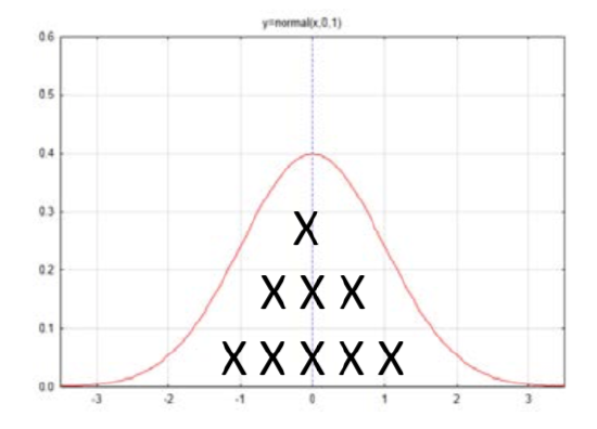
The mean of this distribution is found from \(\mu = np\). The standard deviation is \(\sigma = \sqrt{npq}\). The formula for determining the number of standard deviations a value is from the mean is \(z = \dfrac{x - \mu}{\sigma}\).
Counts were eventually turned into proportions by dividing the counts by the sample size. The distribution consisted of all the possible sample proportions.
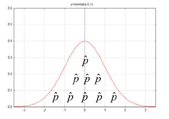
The distribution of sample proportions has a mean of \(\mu_{\hat{p}} = p\) and a standard deviation of \(\sigma_{\hat{p}} = \dfrac{p(1 - p)}{n}\). The formula for determining the number of standard deviations a sample proportion is from the mean is \(z = \dfrac{\hat{p} - p}{\sqrt{\dfrac{p(1 - p)}{n}}}\).
The next time we encountered the normal distribution was when we had quantitative data in which case the distribution was made up of sample means.
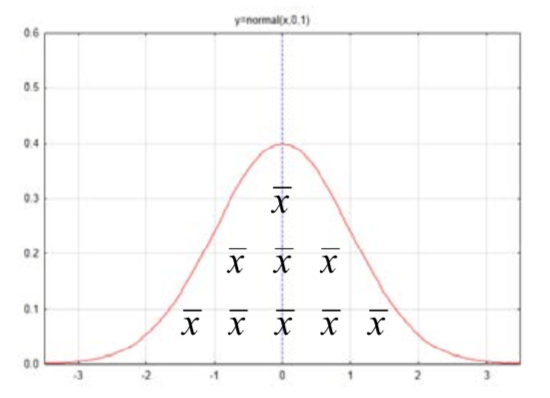
The mean of all possible sample means is \(\mu_{\bar{x}} = \mu\) and the standard error is \(\sigma_{\bar{x}} = \dfrac{\sigma}{\sqrt{n}}\). The formula for determining the number of standard deviations a sample mean is from the hypothesized population mean is \(z = \dfrac{\bar{x} - \mu}{\dfrac{\sigma}{\sqrt{n}}}\). Because \(\sigma\) is not known, it is estimated with s, so that the estimated standard error is \(s_{\bar{x}} = \dfrac{s}{\sqrt{n}}\) and the Z formula is replaced by the t formula where \(t = \dfrac{\bar{x} - \mu}{\dfrac{s}{\sqrt{n}}}\).
The distributions and formulas that were just shown are the same as, or similar to, the ones that you saw in Chapter 5 and that are appropriate for questions 1, 3, and 4. On the other hand, questions 2 and 5 have hypotheses unlike those encountered before and so some effort is needed to define the relevant distributions and their means and standard deviations. These will be based on three statistical results that will not be proven here:
1. The mean of the difference of two random variables is the difference of the means.
2. The variance of the difference of two independent random variables is the sum of the variances.
3. The difference of two independent normally distributed random variables is also normally distributed. (Aliaga, Martha, and Brenda Gunderson. Interactive Statistics. Upper Saddle River, NJ: Pearson Prentice Hall, 2006. Print.)
We will start with the question of whether the proportion of people with a health problem such as diabetes, heart disease or cancer is lower for those who meet the government’s exercise recommendation than it is for those who don’t. This means that there are two populations, the population that exercises above government recommended levels and the population that doesn’t. Within each population, the proportion of people with a health problem will be found. A hypothesis test will be used to determine if people who exercise at the recommended levels have fewer health problems than people who don’t. The hypotheses are:
\(H_0: P_{\text{exercise}} = P_{\text{don't}}\)
\(H_1: P_{\text{exercise}} < P_{\text{don't}}\)
Writing hypotheses in this manner is easy to interpret, but an algebraic manipulation of these will give us some insight into the distribution that would be used to represent the null hypothesis. \(P_{\text{don’t}}\) will be subtracted from both sides.
\(H_0: P_{\text{exercise}} - P_{\text{don't}} = 0\)
\(H_1: P_{\text{exercise}} - P_{\text{don't}} < 0\)
Since neither \(P_{\text{exercise}}\) or \(P_{\text{don’t}}\) is known because these are parameters, the best that can be done is estimate them using sample proportions. Therefore \(\hat{p}_{exercise}\) will be used as an estimate of \(P_{\text{exercise}}\) and \(\hat{p}_{don't}\) will be used as an estimate of \(P_{\text{don’t}}\). Then \(\hat{p}_{exercise} - \hat{p}_{don't}\) as an estimate for \(P_{\text{exercise}} - P_{\text{don’t}}\).
The distribution of interest to us is the one consisting of the difference between sample proportions, generically shown as \(\hat{p}_{A} - \hat{p}_{B}\).
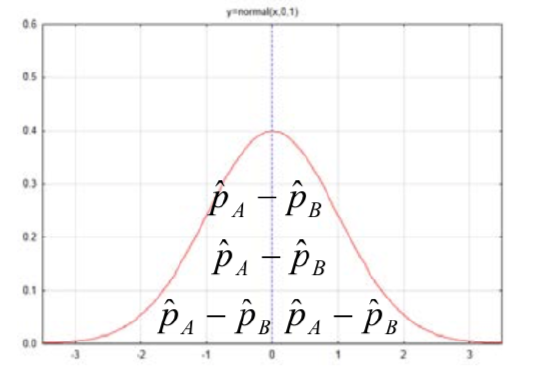
The mean of this distribution is \(p_A - p_B\) and the standard deviation is \(\sqrt{\dfrac{p_{A} (1 - p_{A})}{n_{A}} + \dfrac{p_{B} (1 - p_{B})}{n_{B}}}\). Since the only thing that is known about \(p_A\) and \(p_B\) is that they are equal, it is necessary to estimate their value so that the standard deviation can actually be computed. To do this, the sample proportions will be combined. The combined proportion is defined as
\[\hat{p}_c = \dfrac{x_A + x_B}{n_A + n_B}.\]
Replacing \(p_A\) and \(p_B\) with \(\hat{p}_c\) results in the formula for estimated standard error of
\[\sqrt{\dfrac{\hat{p}_{c} (1 - \hat{p}_{c})}{n_{A}} + \dfrac{\hat{p}_{c} (1 - \hat{p}_{c})}{n_{B}}} \text{ or } \sqrt{\hat{p}_{c} (1 - \hat{p}_{c}) (\dfrac{1}{n_{A}} + \dfrac{1}{n_{B}})}\]
We can now substitute into the \(z\) formula, \(z = \dfrac{x − \mu}{\sigma}\) to get the test statistic used when testing the difference between two population proportions,
\[z = \dfrac{(\hat{p}_{A} - \hat{p}_{B}) - (p_{A} - p_{B})}{\sqrt{\hat{p}_{c} (1 - \hat{p}_{c}) (\dfrac{1}{n_{A}} + \dfrac{1}{n_{B}})}}\]
This can be written a little more simply in cases when the null hypothesis is \(P_A = P_B\) which means that \(p_A – p_B = 0\), so that term can be eliminated to give the test statistic
\[z = \dfrac{(\hat{p}_{A} - \hat{p}_{B})}{\sqrt{\hat{p}_{c} (1 - \hat{p}_{c}) (\dfrac{1}{n_{A}} + \dfrac{1}{n_{B}})}}\]
For this test statistic, both sample sizes should be sufficient large (n>20) with a minimum of 5 successes and 5 failures.
A similar approach will be taken with question 4, which asks if the average amount of exercise a college graduate does in a week is different than someone who does not graduate from college? There are two populations being compared, the population of college graduates and the population of non- college graduates. The average amount of exercise in each of these populations will be compared.
When the means of two populations are compared, the hypotheses are written as:
\(H_0: \mu_{\text{college grad}} = \mu_{\text{not college grad}}\)
\(H_1: \mu_{\text{college grad}} \ne \mu_{\text{not college grad}}\)
Writing hypotheses in this manner is easy to interpret, but an algebraic manipulation of these will give us some insight into the distribution that would be used to represent the null hypothesis.
\(\mu_{\text{not college grad}}\) will be subtracted from both sides.
\(H_0: \mu_{\text{college grad}} - \mu_{\text{not college grad} = 0}\)
\(H_1: \mu_{\text{college grad}} - \mu_{\text{not college grad} \ne 0}\)
Since \(n\) either \(\mu_{\text{college grad}}\) or \(\mu_{\text{not college grad}}\) are known because these are parameters, the best that can be done is to estimate them using sample means. Therefore \(\bar{x}_{college\ grad}\) will be used as an estimate of \(\mu_{\text{college grad}}\) and \(\bar{x}_{college\ grad}\) will be used as an estimate of \(\mu_{\text{not college grad}}\). Then \(\bar{x}_{college\ grad} - \bar{x}_{not\ college\ grad}\)
The distribution of interest to us is the one consisting of the difference between sample means, generically shown as \(\bar{x}_{A} - \bar{x}_{B}\).
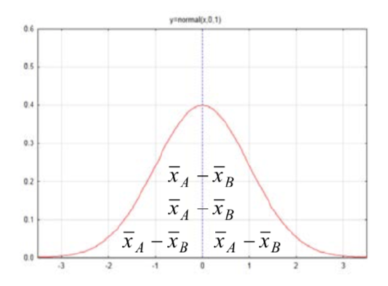
The mean of this distribution is \(\mu_A - \mu_B\) and the standard deviation is \(\sqrt{\dfrac{\sigma_{A}^{2}}{n_{A}} + \dfrac{\sigma_{B}^{2}}{n_{B}}}\). Once again we run into the problem that the standard deviation of the populations \(\sigma_A\) and \(\sigma_B\) are not known, so they must be estimated with the sample standard deviation sA and sB. An additional problem is that it is not known if the variances for the two populations are equal (homogeneous). Unequal variances (heterogeneous) increase the Type I error rate. (Sheskin, David J. Handbook of Parametric and Nonparametric Statistical Procedures. Boca Raton: Chapman & Hall/CRC, 2000. Print.)
The \(t\) Test for Two Independent Samples is used to test the hypothesis. This test is dependent upon the following assumptions.
- Each sample is randomly selected from the population it represents.
- The distribution of data in the population from which the sample was drawn is normal
- The variances of the two populations are equal. This is the homogeneity of variance assumption. (Sheskin, David J. Handbook of Parametric and Nonparametric Statistical Procedures. Boca Raton: Chapman & Hall/CRC, 2000. Print.)
The test statistic follows the same basic pattern as the other tests, which involves finding the number of standard errors a statistic is away from the hypothesized parameter.
\[t = \dfrac{(\bar{x}_{A} - \bar{x}_{B}) - (\mu_A - \mu_B)}{\sqrt{\dfrac{s_{1}^{2}}{n_1} + \dfrac{s_{2}^{2}}{n_2}}}\]
The assumption with this formula is that the two sample sizes are equal. If this formula is used when the sample sizes are not equal, there is an increased chance of making a Type I error. In such cases, an alternative formula is used which includes the weighted average of the estimated population variances of the two groups. The weighted average is based on the number of degrees of freedom in each sample. This formula can be used for both equal and non-equal sample sizes.
\[t = \dfrac{(\bar{x}_{A} - \bar{x}_{B}) - (\mu_A - \mu_B)}{\sqrt{[\dfrac{(n_A - 1)s_{A}^{2} + (n_B - 1)s_{B}^{2}}{n_A + n_B - 2}][\dfrac{1}{n_A} + \dfrac{1}{n_B}]}}\]
Because two parameters (\(\sigma_A\) and \(\sigma_B\)) are replaced by \(s_A\) and \(s_B\), two degrees of freedom are lost. Thus, the number of degrees of freedom for this test statistic is \(n_1 + n_2 - 2\).
There are four different hypothesis tests presented in this chapter. The hypotheses and test statistics are summarized in the following table.
| Proportions (for categorical data) | Means (for quantitative data) | |
| 1 - sample | \(H_0: p = p_0\) \(H_1: p < p_0\) or \(p > p_0\) or \(p \ne p_0\) \(z = \dfrac{\hat{p} - p}{\sqrt{\dfrac{p(1 - p)}{n}}}\) Assumptions: \(np \ge 5, n(1 - p) \ge 5\) |
\(H_0: \mu = \mu_0\) \(H_1: \mu < \mu_0\) or \(\mu > \mu_0\) or \(\mu \ne \mu_0\) \(t = \dfrac{\bar{x} - \mu}{\dfrac{s}{\sqrt{n}}}\) df = n - 1 Assumptions: If \(n < 30\), population is approximately normally distributed. |
| 2 - samples | \(H_0: p_A = p_B\) \(H_1: p_A < p_B\) or \(p_A > p_B\) or \(p_A \ne p_B\) \(z = \dfrac{(\hat{p}_{A} - \hat{p}_{B}) - (p_{A} - p_{B})}{\sqrt{\hat{p}_{c} (1 - \hat{p}_{c}) (\dfrac{1}{n_{A}} + \dfrac{1}{n_{B}})}}\) where \(\hat{p}_c = \dfrac{x_A + x_B}{n_A + n_B}\) Assumptions: \(np \ge 5\), \(n(1 - p) \ge 5\) for both populations |
\(H_0: \mu_A = \mu_B\) \(H_1: \mu_A < \mu_B\) or \(\mu_A > \mu_B\) or \(\mu_A \ne \mu_B\) \(t = \dfrac{(\bar{x}_{A} - \bar{x}_{B}) - (\mu_A - \mu_B)}{\sqrt{[\dfrac{(n_A - 1)s_{A}^{2} + (n_B - 1)s_{B}^{2}}{n_A + n_B - 2}][\dfrac{1}{n_A} + \dfrac{1}{n_B}]}}\) df = \(n_A + n_B - 2\) Assumptions: If \(n < 30\), population is approximately normally distributed. |
For each hypothesis-testing situation, you will have to decide which formula and which table to use. Notice that when the hypotheses are about proportions, the standard normal \(z\) distribution is used. When the hypotheses are about means, the t distributions are used.
We will now return to our original five questions. The statistics given in this problem are fictitious.
- Is the proportion of people who exercise enough to meet the government’s recommendation less than 0.25?
Assume that a random sample of 800 adults was taken. Of these, 184 claimed they met the government’s recommendation for exercise. Can we conclude that the proportion that meets this recommendation is less than 25%? Use a level of significance of 0.05.
The hypotheses are:
\(H_0: p = 0.25\)
\(H_1: p < 0.25\)
The sample proportion is \(\bar{p} = \dfrac{x}{n} = \dfrac{184}{800} = 0.23\)
The test statistic is \(z = \dfrac{\hat{p} - p}{\sqrt{\dfrac{p(1 - p)}{n}}}\). With substitution \(z = \dfrac{0.23 - 0.25}{\sqrt{\dfrac{0.25(1 - 0.25)}{800}}} = -1.31\)
Check the standard normal distribution table to find the area to the left is 0.0951. This is the p-value because the direction of the extreme is to the left. Since the p-value is greater than the level of significance, the data are consistent with the null hypothesis. We conclude that at the 0.05 level of significance, the proportion of adults who meet government recommendations for exercise is not significantly less than 25% (\(z\) = -1.31, \(p\) = 0.0951, \(n\) = 800). - Is the proportion of people with a health problem such as diabetes, heart disease or cancer lower for those who meet the government’s exercise recommendation than it is for those who don’t?
Assume a random sample is taken from both populations. For the people who meet the recommended amount of exercise, 84 out of 560 had a health problem. For the people who did not exercise enough, 204 out of 850 had a health problem.
The hypotheses are:
\(H_0: P_{\text{exercise}} = P_{\text{don't}}\)
\(H_1: P_{\text{exercise}} < P_{\text{don't}}\)
The sample proportions are \(\hat{p}_{exercise} = \dfrac{x}{n} = \dfrac{84}{560} = 0.15\) and \(\hat{p}_{don't} = \dfrac{x}{n} = \dfrac{204}{850} = 0.24\)
The pooled proportion is \(\hat{p}_{c} = \dfrac{x_{A} + x_{B}}{n_{A} + n_{B}} = \dfrac{84 + 204}{560 + 850} = 0.204\)
The test statistic is \(z = \dfrac{(\hat{p}_{A} - \hat{p}_{B}) - (p_{A} - p_{B})}{\sqrt{\hat{p}_{c} (1 - \hat{p}_{c}) (\dfrac{1}{n_{A}} + \dfrac{1}{n_{B}})}}\)
with substitution \(z = \dfrac{(0.15 - 0.24)}{\sqrt{0.204(1 - 0.204) (\dfrac{1}{560} + \dfrac{1}{850})}} = -4.10\)
Checking the standard normal distribution table, the \(z\) value of -4.10 is below the lowest value in the table (-3.49) therefore the area in the left tail is less than 0.0002. We conclude that at the 0.05 level of significance, the proportion of health problems for people meeting the government’s recommendation for exercise is significant less than for people who don’t exercise this much (\(z\) = -4.10, p < 0.0002, \(n_{\text{exercise}}=560\), \(n_{\text{don’t}} = 850\)). - Is the average amount of exercise a college student does in a week greater than 2.5 hours?
For this question, the evidence that needs to be gathered is hours of exercise in a week. That is quantitative data. To use the t-test, we need to make sure the data in the sample are approximately normally distributed. The hypotheses that will be tested are:
\(H_0: \mu = 2.5\)
\(H_1: \mu > 2.5\)
The level of significance is 0.10.
The number of hours of exercise by 20 randomly selected students is shown in the table below.3.7 2 7.1 1.7 0 0 2.1 2.9 4 3.2 3.4 1.3 1 4.2 0 1.3 2.9 5.3 4.4 2.3 A histogram for this data shows that it is approximately normally distributed. The biggest deviation from normality is in the left tail since it isn’t possible to exercise less than 0 hours per week.
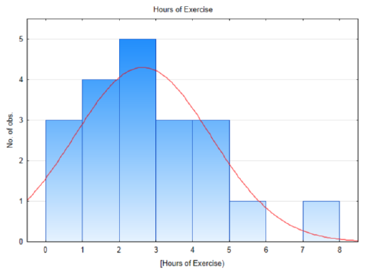
The sample mean and standard deviation are 2.64 hours and 1.855 hours, respectively. The test statistic is: \(t = \dfrac{\bar{x} - \mu}{\dfrac{s}{\sqrt{n}}}\), with substitution, \(t = \dfrac{2.64 - 2.5}{\dfrac{1.855}{\sqrt{20}}}\). After simplification, t = 0.338. There are 19 degrees of freedom (20 – 1) . Use the t table, in the row with 19 degrees of freedom, find the location of 0.338. An excerpt of the table is shown below. Notice that 0.338 falls between 0.257 and 0.688 so consequently the table shows that the area in the right tail is between 0.25 and 0.40. Since the level of significance is 0.1, and since the area in the tail is greater than 0.1 and more specifically greater than 0.25, we would report that the p-value is greater than 0.25.

Conclusion: at the 0.10 level of significance, the average time that college students exercise is not significantly greater than 2.5 hours (\(t\) = 0.338, \(p\) > 0.25, \(n\) = 20). - Is the average weight of a person less after a month of new regular aerobic fitness program?
For this question, two sets of data must be collected, the before weight and the after weight. The before weight will be subtracted from the after weight to determine the change in weight. Because ultimately there will be only one set of data, the t test for one population mean will be used.
\(H_0: \mu = 0\)
\(H_1: \mu < 0\)
The level of significance is 0.10.Subject 1 2 3 4 5 6 7 8 9 Before weight 158 213 142 275 184 136 172 263 205 After weight 154 213 135 278 180 134 171 258 199 After Before -4 0 -7 3 -4 -2 -1 -5 -6 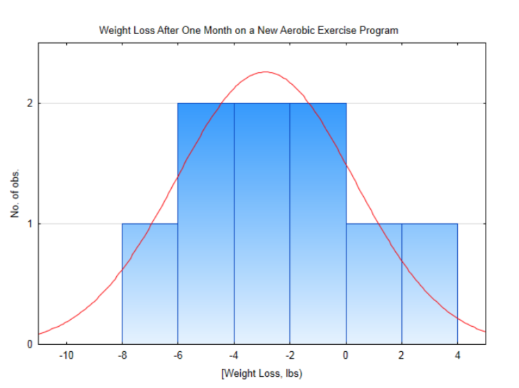
This distribution is approximately normal, so it is appropriate to use the t-test for one population mean. The sample mean is -2.89 lbs with a standard deviation of 3.18 lbs. The test statistic is: \(t = \dfrac{\bar{x} - \mu}{\dfrac{s}{\sqrt{n}}}\), with substitution, \(t = \dfrac{-2.89 - 0}{\dfrac{3.18}{\sqrt{9}}}\). After simplification, t = -2.726. There are 8 degrees of freedom (9-1). Since -2.726 falls between 2.306 and 2.896 in the row for 8 degrees of freedom and since the level of significance is 0.1 but the area in the tail to the left of -2.726 is less than 0.025, then the conclusion is that the new weight is significantly less than the original weight (\(t\) = -2.726, \(p\) < 0.025, \(n\) = 9). We conclude people lost weight.

- For those who exercise regularly, is the average amount of exercise a college graduate does in a week different than someone who does not graduate from college?
Assume a random sample is taken for the population of college graduates who exercise regularly and a different random sample is taken from the population of non-graduates who exercise regularly. Also assume that the amount of exercise is normally distributed for both groups and that the variance is homogeneous. The hypotheses are shown below. Use a level of significance of 0.05.
\(H_0: \mu_{\text{college grad}} = \mu_{\text{not college grad}}\)
\(H_1: \mu_{\text{college grad}} \ne \mu_{\text{not college grad}}\)
The table below shows the mean, standard deviation and sample size for the two samples.Units: hours/week College Graduates Not College Graduations Mean 4.2 3.8 Standard Deviation 1.3 1.2 Sample size, \(n\) 12 16 The difference in sample size means that we need the test statistic formula:
\(t = \dfrac{(\bar{x}_{A} - \bar{x}_{B}) - (\mu_A - \mu_B)}{\sqrt{[\dfrac{(n_A - 1)s_{A}^{2} + (n_B - 1)s_{B}^{2}}{n_A + n_B - 2}][\dfrac{1}{n_A} + \dfrac{1}{n_B}]}}\)
which is used for independent populations. Substituting into the formula gives:
\(t = \dfrac{(4.2 - 3.8) - (0)}{\sqrt{[\dfrac{(12 - 1) 1.3^{2} + (16 - 1) 1.2^{2}}{12 + 16 - 2}][\dfrac{1}{12} + \dfrac{1}{16}]}} = 0.842\)
Because of the inequality sign in the alternative hypothesis, this is a two-tailed test. The test statistic of 0.842 produces a p-value between 0.5 and 0.8. Since this is clearly higher than the level of significance, the conclusion is that at the 0.05 level of significance, the amount of exercise for college graduates is not significantly different than the amount for non-graduates (\(t\) = 0.842, \(p\) > 0.5, \(n_{\text{college grads}} =12\), \(n_{\text{not college grads}} =16\)). 
The t-test for two independent samples has been based on the assumption of homogeneity of variance. There are tests to determine if the variance is homogeneous and modifications that can be made to the degrees of freedom if it isn’t. These are not included in this text.
All of these tests can be done using the TI84 calculator. The tests are found by selecting the STAT key and then using the cursor arrows to move to the right to TESTS.
| Proportions (for categorical data) | Means (for quantitative data) | |
| 1 - sample | \(H_0: p = p_0\) \(H_1: p < p_0\) or \(p > p_0\) or \(p \ne p_0\) Test 5: 1- PropZTest |
\(H_0: \mu = \mu_0\) \(H_1: \mu < \mu_0\) or \(mu > \mu_0\) or \(mu \ne \mu_0\) Test 2: T- Test |
| 2 - samples | \(H_0: p_A = p_B\) \(H_1: p_A < p_B\) or \(p_A > p_B\) or \(p_A \ne p_B\) Test 6: 2- PropZTest |
\(H_0: \mu_A = \mu_B\) \(H_1: \mu_A < \mu_B\) or \(\mu_A > \mu_B\) or \(\mu_A \ne \mu_B\) Test 4: 2-SampTTest |


