
4: Inferential Theory
- Page ID
- 5321

\( \newcommand{\vecs}[1]{\overset { \scriptstyle \rightharpoonup} {\mathbf{#1}} } \)
\( \newcommand{\vecd}[1]{\overset{-\!-\!\rightharpoonup}{\vphantom{a}\smash {#1}}} \)
\( \newcommand{\dsum}{\displaystyle\sum\limits} \)
\( \newcommand{\dint}{\displaystyle\int\limits} \)
\( \newcommand{\dlim}{\displaystyle\lim\limits} \)
\( \newcommand{\id}{\mathrm{id}}\) \( \newcommand{\Span}{\mathrm{span}}\)
( \newcommand{\kernel}{\mathrm{null}\,}\) \( \newcommand{\range}{\mathrm{range}\,}\)
\( \newcommand{\RealPart}{\mathrm{Re}}\) \( \newcommand{\ImaginaryPart}{\mathrm{Im}}\)
\( \newcommand{\Argument}{\mathrm{Arg}}\) \( \newcommand{\norm}[1]{\| #1 \|}\)
\( \newcommand{\inner}[2]{\langle #1, #2 \rangle}\)
\( \newcommand{\Span}{\mathrm{span}}\)
\( \newcommand{\id}{\mathrm{id}}\)
\( \newcommand{\Span}{\mathrm{span}}\)
\( \newcommand{\kernel}{\mathrm{null}\,}\)
\( \newcommand{\range}{\mathrm{range}\,}\)
\( \newcommand{\RealPart}{\mathrm{Re}}\)
\( \newcommand{\ImaginaryPart}{\mathrm{Im}}\)
\( \newcommand{\Argument}{\mathrm{Arg}}\)
\( \newcommand{\norm}[1]{\| #1 \|}\)
\( \newcommand{\inner}[2]{\langle #1, #2 \rangle}\)
\( \newcommand{\Span}{\mathrm{span}}\) \( \newcommand{\AA}{\unicode[.8,0]{x212B}}\)
\( \newcommand{\vectorA}[1]{\vec{#1}} % arrow\)
\( \newcommand{\vectorAt}[1]{\vec{\text{#1}}} % arrow\)
\( \newcommand{\vectorB}[1]{\overset { \scriptstyle \rightharpoonup} {\mathbf{#1}} } \)
\( \newcommand{\vectorC}[1]{\textbf{#1}} \)
\( \newcommand{\vectorD}[1]{\overrightarrow{#1}} \)
\( \newcommand{\vectorDt}[1]{\overrightarrow{\text{#1}}} \)
\( \newcommand{\vectE}[1]{\overset{-\!-\!\rightharpoonup}{\vphantom{a}\smash{\mathbf {#1}}}} \)
\( \newcommand{\vecs}[1]{\overset { \scriptstyle \rightharpoonup} {\mathbf{#1}} } \)
\(\newcommand{\longvect}{\overrightarrow}\)
\( \newcommand{\vecd}[1]{\overset{-\!-\!\rightharpoonup}{\vphantom{a}\smash {#1}}} \)
\(\newcommand{\avec}{\mathbf a}\) \(\newcommand{\bvec}{\mathbf b}\) \(\newcommand{\cvec}{\mathbf c}\) \(\newcommand{\dvec}{\mathbf d}\) \(\newcommand{\dtil}{\widetilde{\mathbf d}}\) \(\newcommand{\evec}{\mathbf e}\) \(\newcommand{\fvec}{\mathbf f}\) \(\newcommand{\nvec}{\mathbf n}\) \(\newcommand{\pvec}{\mathbf p}\) \(\newcommand{\qvec}{\mathbf q}\) \(\newcommand{\svec}{\mathbf s}\) \(\newcommand{\tvec}{\mathbf t}\) \(\newcommand{\uvec}{\mathbf u}\) \(\newcommand{\vvec}{\mathbf v}\) \(\newcommand{\wvec}{\mathbf w}\) \(\newcommand{\xvec}{\mathbf x}\) \(\newcommand{\yvec}{\mathbf y}\) \(\newcommand{\zvec}{\mathbf z}\) \(\newcommand{\rvec}{\mathbf r}\) \(\newcommand{\mvec}{\mathbf m}\) \(\newcommand{\zerovec}{\mathbf 0}\) \(\newcommand{\onevec}{\mathbf 1}\) \(\newcommand{\real}{\mathbb R}\) \(\newcommand{\twovec}[2]{\left[\begin{array}{r}#1 \\ #2 \end{array}\right]}\) \(\newcommand{\ctwovec}[2]{\left[\begin{array}{c}#1 \\ #2 \end{array}\right]}\) \(\newcommand{\threevec}[3]{\left[\begin{array}{r}#1 \\ #2 \\ #3 \end{array}\right]}\) \(\newcommand{\cthreevec}[3]{\left[\begin{array}{c}#1 \\ #2 \\ #3 \end{array}\right]}\) \(\newcommand{\fourvec}[4]{\left[\begin{array}{r}#1 \\ #2 \\ #3 \\ #4 \end{array}\right]}\) \(\newcommand{\cfourvec}[4]{\left[\begin{array}{c}#1 \\ #2 \\ #3 \\ #4 \end{array}\right]}\) \(\newcommand{\fivevec}[5]{\left[\begin{array}{r}#1 \\ #2 \\ #3 \\ #4 \\ #5 \\ \end{array}\right]}\) \(\newcommand{\cfivevec}[5]{\left[\begin{array}{c}#1 \\ #2 \\ #3 \\ #4 \\ #5 \\ \end{array}\right]}\) \(\newcommand{\mattwo}[4]{\left[\begin{array}{rr}#1 \amp #2 \\ #3 \amp #4 \\ \end{array}\right]}\) \(\newcommand{\laspan}[1]{\text{Span}\{#1\}}\) \(\newcommand{\bcal}{\cal B}\) \(\newcommand{\ccal}{\cal C}\) \(\newcommand{\scal}{\cal S}\) \(\newcommand{\wcal}{\cal W}\) \(\newcommand{\ecal}{\cal E}\) \(\newcommand{\coords}[2]{\left\{#1\right\}_{#2}}\) \(\newcommand{\gray}[1]{\color{gray}{#1}}\) \(\newcommand{\lgray}[1]{\color{lightgray}{#1}}\) \(\newcommand{\rank}{\operatorname{rank}}\) \(\newcommand{\row}{\text{Row}}\) \(\newcommand{\col}{\text{Col}}\) \(\renewcommand{\row}{\text{Row}}\) \(\newcommand{\nul}{\text{Nul}}\) \(\newcommand{\var}{\text{Var}}\) \(\newcommand{\corr}{\text{corr}}\) \(\newcommand{\len}[1]{\left|#1\right|}\) \(\newcommand{\bbar}{\overline{\bvec}}\) \(\newcommand{\bhat}{\widehat{\bvec}}\) \(\newcommand{\bperp}{\bvec^\perp}\) \(\newcommand{\xhat}{\widehat{\xvec}}\) \(\newcommand{\vhat}{\widehat{\vvec}}\) \(\newcommand{\uhat}{\widehat{\uvec}}\) \(\newcommand{\what}{\widehat{\wvec}}\) \(\newcommand{\Sighat}{\widehat{\Sigma}}\) \(\newcommand{\lt}{<}\) \(\newcommand{\gt}{>}\) \(\newcommand{\amp}{&}\) \(\definecolor{fillinmathshade}{gray}{0.9}\)Prior to elections, pollsters will survey approximately 1000 people and on the basis of their results, try to predict the outcome of the election. On the surface, it should seem like an absurdity that the opinions of 1000 can give any indication about the opinion of 100,000,000 voters in a national presidential election. Likewise, taking 100 or 1000 water samples from the Puget Sound, when that is a miniscule amount of water compared to the total amount of constantly changing water in the Sound, should seem insufficient for making a decision.
The objective of this chapter is to develop the theory that helps us understand why a relatively small sample size can actually lead to conclusions about a much larger population. The explanation is different for categorical and quantitative data. We will begin with categorical data.
The journey that you will take through this section has a final destination at the formula that will ultimately be used to test hypotheses. While you might be willing to accept the formula without taking the journey, it will be the journey that gives meaning to the formula. Because data are stochastic, that is, they are subject to randomness, probability plays a critical role in this journey.
Our journey begins with the concept of inference. Inference means that a small amount of observed information is used to draw general conclusions. For example, you may visit a business and receive outstanding customer service from which you infer that this business cares about its customers. Inference is used when testing a hypothesis. A small amount of information, the sample, is used to draw a conclusion, or infer something about the entire population.
The theory begins with finding the probability of getting a particular sample and ultimately ends with creating distributions of all the sample results that are possible if the null hypothesis is true. For each step of the 7-step journey, digressions will be made to learn about the specific rules of probability that contribute to the inferential theory.
Before starting, it is necessary to clarify some of the terminology that will be used. Regardless of the question being asked, if it produces categorical data, that data will be identified generically as a success or failure, without using those terms in their customary manner. For example, a researcher making a hypothesis about the proportion of people who are unemployed would consider being unemployed a success from the statistical point of view, and being employed as a failure, even though that contradicts the way it is viewed in the real world. Thus, success is data values about which the hypotheses are written and failure is the alternate data value.
Briefing 4.1 Self-driving Cars
Google, as well as most car companies, are developing self-driving cars. These autonomous cars will not need to have a driver and are considered less likely to be in an accident than cars driven by humans. Cars such as these are expected to be available to the public around the years 2020 – 2025. There are many questions that must be answered before these cars are made available. One such question is to determine who is responsible in the event of an accident. Is the owner of the car responsible, even though they were not steering the car or is the manufacturer responsible since their technology did not avoid the accident? (mashable.com/2014/07/07/drive...-cars-tipping- point/, viewed July 2014).
Step 1 – How likely is it that a particular data value is success?
Suppose a researcher wanted to determine the proportion of the public that believe the owner is responsible for the accident. The researcher has a hypothesis that the proportion is over 60%. In this case, the hypotheses will be:
- \(H_0: p = 0.60\)
- \(H_1: p > 0.60\)
When collecting data, the order in which the units or people are selected determines the order in which the data is collected. In this case, assigning responsibility to the owner will be considered a success and assigning responsibility to the manufacturer is considered a failure. If the first person believes the owner is responsible, the second person believes the manufacturer is responsible, the third person selects the manufacturer, the fourth, fifth and sixth people all select the owner as the responsible party, then we can convert this information to successes and failure by listing the order in which the data were obtained as SFFSSS.
The strategy that is employed to determine which of two competing hypotheses is better supported is always to assume that the null hypothesis is true. This is a critical point, because if we can assume a condition is true, then we can determine the probability of getting our particular sample result, or more extreme results. This is a p-value.
However, before we can determine the probability of obtaining a sequence such as SFFSSS, we must first find the probability of obtaining a success. For this, we need to explore the concept of probability.
Digression 1 – Probability
Probability is the chance that a particular outcome will happen if a process is repeated a very large number of times. It is quantified by dividing the number of favorable outcomes by the number of possible outcomes. This is shown as a formula:
\[P(A) = \dfrac{\text{Number of Favorable Outcomes}}{\text{Number of Possible Outcomes}}\]
where \(P(A)\) means the probability of some event called \(A\). This formula assumes that all outcomes are equally likely, which is what happens with a good random sampling process. The entire set of possible outcomes is called the sample space. The number of possible outcomes is the same as the number of elements in the sample space.
While the intent of this chapter is to focus on developing the theory to test hypotheses, a few concepts will be explained initially with easier examples.
If we wanted to know the probability of getting a tail when we flip a fair coin, then we must first consider the sample space, which would be {H, T}. Since there is one element in that sample space that is favorable and the sample space contains two elements, the probability is \(p(tails) = \dfrac{1}{2}\).
To find the probability of getting a 4 when rolling a fair die, we create the sample space with six elements {1,2,3,4,5,6}, since these are the possible results that can be obtained when rolling the die. To find the probability or rolling a 4, we can substitute into the formula to get \(P(4) = \dfrac{1}{6}\).
A more challenging question is to determine the probability of getting two heads when flipping two coins or flipping one coin twice. The sample space for this experiment is {HH, HT, TH, TT}. The probability is (HH) = \(\dfrac{1}{4}\). The probability of getting one head and one tail, in any order is (1 head and 1 tail) = \(\dfrac{2}{4}\) = \(\dfrac{1}{2}\).
Probability will always be a number between 0 and 1, thus \(0 \le P(A) \le 1\). A probability of 0 means something cannot happen. A probability of 1 is a certainty.
Apply this concept of probability to the hypothesis about the responsibility for a self-driving car in an accident.
If we assume that the null hypothesis is true, then the proportion of people who believe the owner is responsible is 0.60. What does that mean? It means that if there are exactly 100 people, then exactly 60 of them hold the owner responsible and 40 of them do not.
If our goal is to find the probability of SFFSSS, then we must first find the probability of getting a success (owner). If there are 100 people in the population and 60 of these select the owner, then the probabiltiy of selecting a person who chooses the owner is \(P(owner) = \dfrac{60}{100} = 0.60\). Notice that this probability exactly equals the proportion defined in the null hypothesis. This is not a coincidence and it will happen every time because the proportion in the null hypothesis is used to generate a theoretical population, which was used to find the probability. The first important step in the process of testing a hypothesis is to realize that the probability of any data being a success is equal to the proportion defined in the null hypothesis, assuming that sampling is done with replacement, or that the population size is extremely large so that removing a unit from the population does not change the probability a significant amount.
Example 1
- If \(H_0: p = 0.35\), then the probability the \(5^{\text{th}}\) value is a success is 0.35.
- If \(H_0: p = 0.82\), then the probability the \(20^{\text{th}}\) value is a success is 0.82.
Step 2 - How likely is it that a particular data value is a failure?
Now that we know how to find the probability of success, we must find the probability of failure. For this, we will again digress to the rules of probability.
Digression 2 - Probability of A or B
When one unit is selected from a population, there can be several possible measures that can be taken on it. For example, a new piece of technology could be put into several brands of cars and then tested for reliability. The contingency table below shows the number of cars in each of the categories. These numbers are fictitious and we will pretend it is the entire population of cars under development.
| Hyundai | Nissan | Total | ||
|---|---|---|---|---|
| Reliable | 80 | 75 | 90 | 245 |
| Not Reliable | 25 | 10 | 20 | 55 |
| Total | 105 | 85 | 110 | Grand Total 300 |
From this we can ask a variety of probability questions.
If one car is randomly selected, what is the probability that it is a Nissan?
\(P(Nissan) = \dfrac{85}{300} = 0.283\)
If one car is randomly selected, what is the probability that the piece of technology was not reliable?
\(P(not reliable) = \dfrac{55}{300} = 0.183\)
If one car is randomly selected, what is the probability that it is a Hyundai or the piece of technology was reliable?
This question introduces the word “or” which means that the car has one characteristic or the other characteristic or both. The word “or” is used when only one selection is made. The table below should help you understand how the formula will be derived.
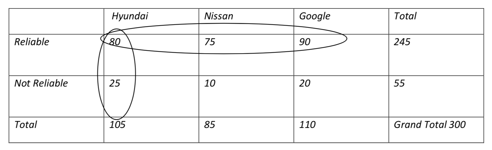
Notice that the 2 values in the Hyundai column are circled and the three values in the Reliable row are circled, but that the value in the cell containing the number 80 that represents the Hyundai and Reliable is circled twice. We don’t want to count those particular cars twice so after adding the column for Hyundai to the row for Reliable, it is necessary to subtract the cell for Hyundai and Reliable because it was counted twice but should only be counted once. Thus, the equation becomes:
P(Hyundai or Reliable) = P(Hyundai) + P(Reliable) – P(Hyundai and Reliable)
= \(\dfrac{105}{300} + \dfrac{245}{300} - \dfrac{80}{300} = \dfrac{270}{300} = 0.90\)
From this we will generalize the formula to be
\[P(A\ or\ B) = P(A) + P(B) - P(A\ and\ B).\]
What happens if we use the formula to determine the probability of randomly selecting a Nissan or a Google car?
Because these two criteria cannot both happen at the same time, they are said to be mutually exclusive. Consequently, their intersection is 0.
P(Nissan or Google) = P(Nissan) + P(Google) – P(Nissan and Google)
= \(\dfrac{85}{300} + \dfrac{110}{300} - \dfrac{0}{300} = \dfrac{195}{300} = 0.65\)
Because the intersection is 0, this leads to a modified formula for categorical data values that are mutually exclusive.
\[P(A\ or\ B) = P(A) + P(B)\]
This is the formula that is of primary interest to us for determining how to find the probability of failure.
If success and failure are the only two possible results, and it is not possible to simultaneously have success and failure, then they are mutually exclusive. Furthermore, if a random selection is made, than it is certain that it will be a success or failure. Things that are certain have a probability of 1. Therefore, we can write the formula using S and F as:
\(P(S\ or\ F) = P(S) + P(F)\)
or
\(1 = P(S) + P(F)\)
with a little algebra this becomes
\[1- P(S) = P(F)\]
What this means is that subtracting the probability of success from 1 gives the probability of failure. The probability of failure is called the complement of the probability of success.
Apply this concept of probability to the hypothesis about the responsibility for a self-driving car in an accident.
Recall that the original hypothesis for the responsibility in an accident is that: H0: p = 0.60. We have established that the probability of success is 0.60. The probability of failure is 0.40 since it is the complement of the probability of success and 1 – 0.60 = 0.40.
Example 2
- If \(H_0: p = 0.35\), then the probability the \(5^{\text{th}}\) value is a success is 0.35. The probability the \(5^{\text{th}}\) value is a failure is 0.65.
- If \(H_0: p = 0.82\), then the probability the \(20^{\text{th}}\) value is a success is 0.82. The probability the \(20^{\text{th}}\) value is a failure is 0.18.
Step 3 - How likely is it that a sample consists of a specific sequence of successes and failures?
We now know that the probability of success is identical to the proportion defined by the null hypothesis and the probability of failure is the complement. But these probabilities apply to only one selection. What happens when more than one is selected? To find that probability, we must learn the last of the probability rules:
\[P(A\ and\ B) = P(A)P(B)\]
Digression 3 - P(A and B) = P(A)P(B)
If two or more selections are made, the word “and” becomes important because it indicates we are seeking one result for the first selection and one result for the second selection. This probability is found by multiplying the individual probabilities. Part of the key to choosing this formula is to identify the problem as an “and” problem. For instance, early in this chapter we found the probability of getting two heads when flipping two coins is 0.25. This problem can be viewed as an “and” problem if we ask “what is the probability of getting a head on the first flip and a head on the second flip”? Using subscripts of 1 and 2 to represent the first and second flips respectively, we can rewrite the formula to show:
\(P(H_1\ and\ H_2) = P(H_1)P(H_2) = (\dfrac{1}{2})(\dfrac{1}{2}) = \dfrac{1}{4} = 0.25.\)
Suppose the researcher randomly selects three cars. What is the probability that there will be one car of each of the makes (Hyundai, Nissan, Google)?
| Hyundai | Nissan | Total | ||
|---|---|---|---|---|
| Reliable | 80 | 75 | 90 | 245 |
| Not Reliable | 25 | 10 | 20 | 55 |
| Total | 105 | 85 | 110 | Grand Total 300 |
First, since there are three cars being selected, this should be recognized as an “and” problem and can be phrased P(Hyundai and Nissan and Google). Before we can determine the probability however, there is one important question that must be asked. That question is whether the researcher will select with replacement.
If the researcher is sampling with replacement, then the probability can be determined as follows.
P(Hyundai and Nissan and Google) = P(Hyundai)P(Nissan)P(Google) =
\((\dfrac{105}{300})(\dfrac{85}{300})(\dfrac{110}{300}) = 0.03636.\)
Notice the slight change in the probability as a result of not using replacement.
Apply this concept of probability to the hypothesis about the responsibility for a self-driving car in an accident.
We are now ready to answer the question of what is the probability that we would get the exact sequence of people if the first person believes the owner is responsible, the second person believes the manufacturer is responsible, the third person selects the manufacturer, the fourth, fifth and sixth people all select the owner as the responsible party. Because there are six people selected, then this is an “and” problem and can be written as P(S and F and F and S and S and S) or more concisely, leaving out the word “and” but retaining it by implication, we write P(SFFSSS). Remember that P(S) = 0.6 and P(F) = 0.4
P(SFFSSS) = P(S)P(F)P(F)P(S)P(S)P(S) = (0.6)(0.4)(0.4)(0.6)(0.6)(0.6) = 0.0207.
To summarize, if the null hypothesis is true, then 60% of the people believe the owner is responsible for accidents. Under these conditions, if a sample of six people is taken, with replacement, then the probability of getting this exact sequence of successes and failures is 0.0207.
Step 4 - How likely is it that a sample would contain a specific number of successes?
Knowing the probability of an exact sequence of successes and failures is not particularly important by itself. It is a stepping-stone to a question of greater importance – what is the probability that four out of six randomly selected people (with replacement) will believe the owner is responsible? This is an important transition in thinking that is being made. It is the transition from thinking about a specific sequence to thinking about the number of successes in a sample.
When data are collected, researchers don’t care about the order of the data, only how many successes there were in the sample. We need to find a way to transition from the probability of getting particular sequence of successes and failures such as SFFSSS to finding the probability of getting four successes from a sample of size 6. This transition will make use of the commutative property of multiplication, the P(A or B) rule and combinatorics (counting methods).
At the end of Step 3 we found that P(SFFSSS) = 0.0207.
- What do you think will be the probability of P(SSSFSF)?
- What do you think will be the probability of P(SSSSFF)?
The answer to both these questions is 0.0207 because all of these sequences contain 4 successes and two failures and since the probability is found by multiplying the probabilities of success and failure in sequence and since multiplication is commutative (order doesn’t matter) then
(0.6)(0.4)(0.4)(0.6)(0.6)(0.6)= (0.6)(0.6)(0.6)(0.4)(0.6)(0.4)= (0.6)(0.6)(0.6)(0.6)(0.4)(0.4) = 0.020736.
If the question now changes from what is the probability of a sequence to what is the probability of 4 successes in a sample of size 6, then we have to consider all the different ways in which four successes can be arranged. We could get 4 successes if the sequence of our selection is SFFSSS or SSSFSF or SSSSFF or numerous other possibilities. Because we are sampling one time and because there are many possible outcomes we could have, this is an “or” problem that uses an expanded version of the formula P(A or B) = P(A) + P(B). This can be written as:
P(4 out of 6) = P(SFFSSS or SSSFSF or SSSSFF or ...) = P(SFFSSS) + P(SSSFSF) + P(SSSSFF) + ...
In other words, we can add the probability of each of these orders. However, since the probability of each of these orders is the same (0.0207) then this process would be much quicker if we simply multiplied 0.0207 by the number of orders that are possible. The question we must answer then is how many ways are there to arrange four successes and 2 failures? To answer this, we must explore the field of combinatorics, which provide various counting methods.
Digression 4 – Combinatorics
Researchers designing the cars will compare different technologies to see which works better. Suppose two brands of a video camera are available for a car. How many different pairs are possible?
A tree-diagram can help explain this.
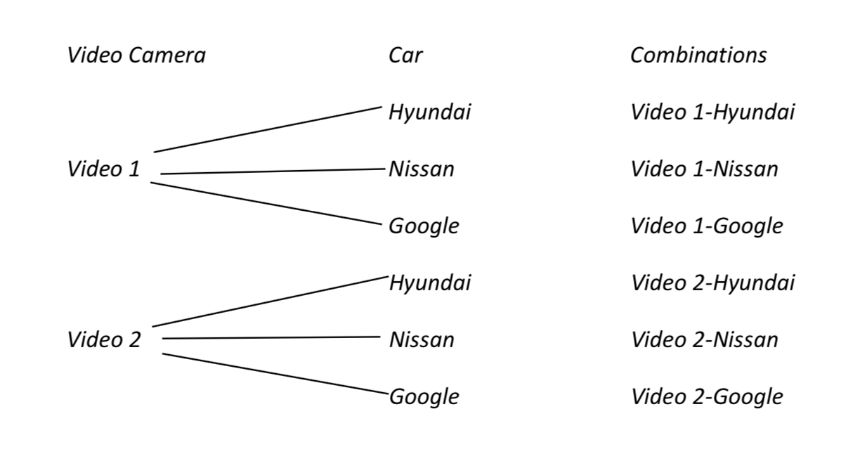
Making a tree-diagram to answer questions such as this can be tedious, so an easier approach is to use the fundamental counting rule which states that if there are M options for one choice that must be made and N options for a second choice that must be made, then there are MN unique combinations. One way to show this is to draw and label a line for each choice that must be made and on the line write the number of options that are available. Multiply the numbers.
_______2_________ ________3_________ = 6
Videos Cars
This tells you there are six unique combinations for one camera and one make of car.
If researchers have 4 test vehicles that will be driving on the freeway as a convoy and the colors of the vehicles are blue, red, green, and yellow, how many ways can these cars be ordered in the convoy?
To answer this question, think of it as having to make four choices, which color of car is first, second, third, fourth. Draw a line for each choice and on the line write the number of options that are available and then multiply these numbers. There are four options for the first car. Once that choice is made there are three options remaining for the second car. When that choice is made, there are two options remaining for the third car. After that choice is made, there is only one option available for the final car.
4 3 2 1 = 24 unique orders
First Car Second Car Third Car Fourth Car
Examples of some of these unique orders include: blue, red, green, and yellow
red, blue, green, and yellow
green, red, blue, and yellow
Each unique sequence is called a permutation. Thus in this situation, there are 24 permutations.
The way to find the number of permutations when all available elements are used is called factorial. In this problem, all four cars are used, so the number of permutations is 4 factorial which is shown symbolically as 4!. 4! means (4)(3)(2)(1). To be more general,
\[n! = n(n - 1)(n - 2)... 1\]
Permutations can also be found when fewer elements are used than are available. For example, suppose the researchers will only use two of the four cars. How many different orders are possible? For example, the blue car followed by the green car is a different order than the green car followed by the blue car. We can answer this question two ways (and hopefully get the same answer both ways!). The first way is to use the fundamental counting rule and draw two lines for the choices we make, putting the number of options available for each choice on the line and then multiplying.
4 3 = 12 permutations
First Car Second Car
Examples of possible permutations include:
Blue, Green, Green, Blue, Blue, Red Yellow, Green
The second approach is to use the formula for permutations when the number selected is less than or equal to the number of available. In this formula, r represents the number of items selected, n represents the number of items available.
\[nPr = \dfrac{n!}{(n - r)!}\]
For this example, n is 4 and r is 2 so with the formula we get:
\(_4P_2 = \dfrac{4!}{(4 - 2)!} = \dfrac{4!}{2!} = \dfrac{4 \cdot 3 \cdot 2 \cdot 1}{2 \cdot 1} = 4 \cdot 3 = 12\) permutations.
Notice the final product of \(4 \cdot 3\) is the same as we have when using the fundamental counting rule. The denominator term of (n-r)! is used to cancel the unneeded numerator terms.
For permutations, order is important, but what if order is not important? For example, what if we wanted to know how many pairs of cars of different colors could be combined if we didn’t care about the order in which they drove. In such a case, we are interested in combinations. While Blue, Green, and Green, Blue represent two permutations, they represent only one combination. There will always be more permutations than combinations. The number of permutations for each combination is r!. That is, when 2 cars are selected there are 2! permutations for each combination.
To determine the number of combinations there are if two of the four cars are selected we can divide the total number of permutations by the number of permutations per combination.
\(Number\ of\ combinations = Number\ of\ permutations (\dfrac{1\ Combination}{Number\ of\ Permutations})\)
Using similar notation as was used for permutations (nPr), combinations can be represented with nCr, so the equation can be rewritten as
\[\begin{array} {rcl} {nCr} &= & {nPr(\dfrac{1}{r!})\ or} \\ {nCr} &= & {\dfrac{n!}{(n - r)!} (\dfrac{1}{r!})} \\ {nCr} &= & {\dfrac{n!}{(n - r)!r!}} \end{array}\]
An alternate way to develop this formula that could be used for larger sample sizes that contain successes and failures is to consider that the number of permutations is n! while the number of permutations for each combination is r!(n-r)!. For example, in a sample of size 20 with 12 successes and 8 failure, there are 20! permutations of the successes and failures combined with 12! permutations of successes and 8! permutations of failures for each combination. Thus,
\(Number\ of\ combinations = 20!(\dfrac{1\ Combination}{12!8!}) = \dfrac{20!}{12!8!}\ or\ as\ a\ formula:\)
\(Number\ of\ combinations = n!(\dfrac{1\ Combination}{r!(n - r)!}) = \dfrac{n!}{r!(n - r)!}\ or\ \dfrac{n!}{(n - r)!r!}\).
For our example about car colors we have:
\(_4C_2 = \dfrac{4!}{(4 - 2)! 2!} = \dfrac{4 \cdot 3 \cdot 2 \cdot 1}{2 \cdot 1 \cdot 2 \cdot 1} = 6\) combinations.
This sequence of combinatorics concepts has reached the intended objective in that the interest is in the number of combinations of successes and failure there are for a given number of successes in a sample. We will now return to the problem of the responsibility for accidents.
Apply this concept of probability to the hypothesis about the responsibility for a self-driving car in an accident.
Recall that 6 people were selected and 4 thought the owner should be responsible. We saw that the probability of any sequence of 4 successes and 2 failures, such as SFFSSS or SSSFSF or SSSSFF is 0.0207 if the null hypothesis is p = 0.60. If we knew the number of combinations of these 4 successes and 2 failures, we could multiply that number times the probability of any specific sequence to get the probability of 4 successes in a sample of size 6.
Using the formula for nCr, we get: \(_6C_4 = \dfrac{6!}{(6 - 4)!4!} = 15\) combinations.
Therefore, the probability of 4 successes in a sample of size 6 is 15*0.020736 = 0.31104. This means that if the null hypothesis of p=0.60 is true and six people are asked, there is a probability of 0.311 that four of those people will believe the owner is responsible.
We are now ready to make the transition to distributions. The following table summarizes our journey to this point.
| Step 1 | Use the null hypothesis to determine P(S) for any selection, assuming replacement. |
| Step 2 | Use the P(A or B) rule to find the complement, which is the P(F) = 1 - P(S) |
| Step 3 | Use the P(A or B) rule to find the probability of a specific sequence of a specific sequence of successes and failures, such as SFFSSS, by multiplying the individual probabilities. |
| Step 4 | Recognize that all combinations of r successes out of a sample of size n have the same probability of occurring. Find the number of combinations nCr and multiply this times the probability of any of the combinations to determine the probability of getting r successes out of a sample of size n. |
Step 5 – How can the exact p-value be found using the binomial distribution?
Recall that in chapter 2, we determined which hypothesis was supported by finding the p-value. If the p-value was small, less than the level of significance, we concluded that the data supported the alternative hypothesis. If the p-value was larger than the level of significance, we concluded that the data supported the null hypothesis. The p-value is the probability of getting the data, or more extreme data, assuming the null hypothesis is true.
In Step 4 we found the probability of getting the data (for example, four successes out of 6) but we haven’t found the probability of getting more extreme data yet. To do so, we must now create distributions. A distribution shows the probability of all the possible outcomes from an experiment. For categorical data, we make a discrete distribution.
Before looking at the distribution that is relevant to the problem of responsibility for accidents, a general discussion of distributions will be provided.
In chapter 4 you learned to make histograms. Histograms show the distribution of the data. In chapter 4 you also learned about means and standard deviations. Distributions have means and standard deviations too.
To demonstrate the concepts, we will start with a simple example. Suppose that someone has two routes used for running. One route is 2 miles long and the other route is 5 miles long. Below is the running schedule for last week.
| Sunday | Monday | Tuesday | Wednesday | Thursday | Friday | Saturday |
| 5 | 2 | 2 | 5 | 2 | 2 | 5 |
A distribution of the amount run each day is shown below.
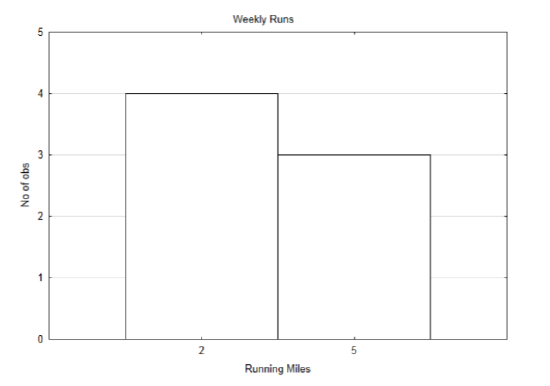
The mean can be found by adding all the daily runs and dividing by 7. The mean is 3.286 miles per day. Because the same distances are repeated on different days, a weighted mean can also be used. In this case, the weight is the number of times a particular distance was run. A weighted mean takes advantage of multiplication instead of addition. Thus, instead of calculating: \(\dfrac{2 + 2 + 2 + 2 + 5 + 5 + 5}{7} = 3.286\). we can multiply each number by the number of times it occurs then divide by the number of occurrences: \(\dfrac{4 \cdot 2 + 3 \cdot 5}{4 + 3} = 3.286\). The formula for a weighted mean is:
\[\dfrac{\sum w \cdot x}{\sum w}\]
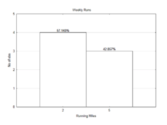
The same graph is presented below, but this time there are percentages above the bars.
Instead of using counts as the weight, the percentages (actually the proportions) can be used as the weight. Thus 57.143% can be written as 0.57143. Likewise, 42.857% can be written 0.42857.
Substituting into the formula gives: \(\dfrac{0.57143 \cdot 2 + 0.42857 \cdot 5}{0.57143 + 0.42857} = 3.286\). Notice that the denominator adds to 1. Therefore, if the weight is the proportion of times that a value occurs, then the mean of a distribution that uses percentages can be found using the formula:
\[\mu = \sum P(x) x\]
This mean, which is also known as the expected value, is the sum of the probability of a value times the value. There is no need for dividing, as is customary when finding means, because we would always just divide by 1.
Recall from chapter 4 that the standard deviation is the square root of the variance. The variance is \(\sigma^2 = \sum[(x - \mu)^2 \cdot P(x)]\). The standard deviation is \(\sigma = \sqrt{\sum[(x - \mu)^2 \cdot P(x)]}\).
\(\sigma = \sqrt{\sum[(x - \mu)^2 \cdot P(x)]}\).
\(\sigma = \sqrt{(2 - 3.286)^2 \cdot 0.57143 + (5 - 3.286)^2 \cdot 0.42857} = 1.485\)
The self-driving car problem will show us one way in which we encounter discrete distributions. In fact, it will result in the creation of a special kind of discrete distribution called the Binomial distribution, which will be defined after exploring the concepts that lead to its creation.
When testing a hypothesis about proportions of successes, there are two random variables that are of interest to us. The first random variable is specific to the data that we will collect. For example, in research about who is responsible for accidents caused by autonomous cars, the random variable would be “responsible party”. There would be two possible values for this random variable, owner or car manufacturer. We have been considering the owner to be a success and the manufacturer to be a failure. The data the researchers collect is about this random variable. However, creating distributions and finding probabilities and p-values requires a shift of our focus to a different random variable. This second random variable is about the number of successes in a sample of size n. In other words, if six people are asked, how many of them think the owner is responsible? It is possible that none of them think the owner is responsible, or one thinks the owner is responsible, or two, or three, or four, or five, or all six think the owner is responsible. Therefore, in a sample of size 6, the random variable for the number of successes can have the values of 0,1,2,3,4,5,6. We have already found that the probability of getting four successes is 0.3110. We will now find the probability of getting 0,1,2,3,5,6 successes, assuming the hypotheses are still \(H_0: p = 0.60\), \(H_1: p > 0.60\). This will allow us to create the discrete binomial distribution of all possible outcomes.
Find the probability of 0 successes
The only way to have 0 successes is to have all failures, thus we are seeking P(FFFFFF).
P(FFFFFF) = P(F)P(F)P(F)P(F)P(F)P(F) = (0.4)(0.4)(0.4)(0.4)(0.4)(0.4) = 0.004096.
Since there is only one combination for 0 successes, then the probability of 0 successes is 0.0041.
Find the probability of 1 success
We know that all combinations have the same probability, so we may as well create the simplest combination for 1 success. This would be SFFFFF.
P(SFFFFF) = P(S)P(F)P(F)P(F)P(F)P(F) = (0.6)(0.4)(0.4)(0.4)(0.4)(0.4) = \((0.6)^{1}(0.4)^{5}\)= 0.006144.
How many combinations are there for 1 success? This can be found using \(_6C_1\).
\(_6C_1 = \dfrac{6!}{(6 - 1)!1!} = 6\) combinations. Does this answer seem reasonable? Consider there are only 6 places in which the success could happen.
The probability of 1 success is then 6*0.006144 = 0.036864 or if we round to four decimal places, 0.0369.
Find the probability of 2 successes.
Instead of doing this problem in steps as was done for the prior examples, it will be demonstrated by combining steps.
\(_6C_2 P\)(SSFFFF)
\(\dfrac{6!}{(6 - 2)! 2!} (0.6)(0.6)(0.4)(0.4)(0.4)(0.4) = \dfrac{6!}{(6 - 2)! 2!} (0.6)^2(0.4)^4 =\)
15(0.009216) = 0.13824 or with rounding to four decimal places 0.1382.
Find the probability of 3 successes using the combined steps. (Now its your turn).
Find the probability of 5 successes.
Find the probability of 6 successes.
When all the probabilities have been found, we can create a table that shows the values the random variable can take and their probabilities. We will define the random variables for the number of successes as X with the possible values defined as x.
| X = x | 0 | 1 | 2 | 3 | 4 | 5 | 6 |
|---|---|---|---|---|---|---|---|
| P(X = x) | 0.0041 | 0.0369 | 0.1382 | 0.2765 | 0.3110 | 0.1866 | 0.0467 |
Do your values for 3,5, and 6 successes agree with the values found in the table?
A graph of this distribution can lead to a better understanding of it. This graph is called a probability mass function, which is shown using a stick graph. It is a way to graph discrete distributions, since there cannot be any values in between the numbers on the x-axis. The heights of the bar correspond to the probability of getting the number of successes.
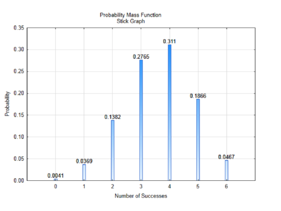
There are three things you should notice about this distribution. First, it is a complete distribution. That is, in a sample of size six, it is only possible to have 0,1,2,3,4,5, or 6 successes and all of those have been included in the graph. The second thing to notice is that all the probabilities have values between 0 and 1. This should be expected because probabilities must always be between 0 and 1. The final thing to notice, which may not be obvious at first, is that if you add all the probabilities, the sum will be 1. The sum of all complete probability distributions should equal 1, \(\sum P(x) =1\). If you add all the probabilities and they don’t equal one, but are very close, it could be because of rounding, not because you did anything wrong.
Digression 5 - Binomial Distributions
The entire journey that has been taken since the beginning of this chapter has led to the creation of a very important discrete distribution called the binomial distribution, which has the following components.
- A Bernoulli Trial is a sample that can have only two possible results, success and failure.
- An experiment can consist of n independent Bernoulli Trials.
- A Binomial Random Variable, X is the number of successes in an experiment
- A Binomial Distribution shows all the values for X and the probability of each of those values occurring.
The assumptions are that:
- All trials are independent.
- The number of trials in an experiment is the same and defined by the variable n.
- The probability of success remains constant for each sample. The probability of failure is the complement of the probability of success. The variable p = P(S) and the variable \(q = P(F). q = 1 – p\).
- The random variable X can have values of 0, 1, 2,...n.
The probability can be found for each possible number of successes that the random variable X can have using the binomial distribution formula
\[P(X = x) = _nC_x P^x q^{n-x}\].
If this formula looks confusing, review the work you did when finding the probability that 3,5 or 6 people believe the owner is responsible, because you were actually using this formula. \(_nC_x\), which is shown in your calculator as \(_nC_r\), is the number of combinations for x successes. The x and the r represent the same thing and are used interchangeably.
p is the probability of success. It comes from the null hypothesis.
q is the probability of failure. It is the complement of p.
n is the sample size
x is the number of successes
If we use this formula for all possible values of the random variable, X, we can create the binomial distribution and graph.
\(P(X = 0) = _6C_0(0.60)^0(0.40)^{6 - 0} = 0.0041\)
\(P(X = 1) = _6C_1(0.60)^1(0.40)^{6 - 1} = 0.0369\)
\(P(X = 2) = _6C_2(0.60)^2(0.40)^{6 - 2} = 0.1382\) You can finish the rest of them.
The TI84 calculator has an easier way to create this distribution. Find and press your Y= key. The cursor should appear in the space next to Y1 = . Next, push the \(2^{\text{nd}}\) key, then the key with VARS on it and DISTR above it. This will take you to the collection of distributions. Scroll up until you find Binompdf. This is the binomial probability distribution function. Select it and then enter the three values n, p, x. For example, if you enter Y1=Binompdf(6,0.60,x) and then select \(2^{\text{nd}}\) TABLE, you should see a table that looks like the following:
X Y1
0 0.0041
1 0.03686
2 0.13824
3 0.27648
4 0.31104
5 0.18662
6 0.04666
If the table doesn't look like this, press \(2^{\text{nd}}\) TBLSET and make sure your settings are:
TblStart = 0
\(\Delta\) TBL = 1
Indpnt: Auto
Depend: Auto.
Binomial distributions have a mean and standard deviation. The approach for finding the mean and standard deviation of a discrete distribution can be applied to a binomial distribution.
| \(X = x\) | 0 | 1 | 2 | 3 | 4 | 5 | 6 |
| \(P(x = x)\) | 0.0041 | 0.0369 | 0.1382 | 0.2765 | 0.3110 | 0.1866 | 0.0467 |
| \(x(P(x))\) | 0 | 0.0369 | 0.2764 | 0.8295 | 1.244 | 0.933 | 0.2802 |
| \((x - \mu)^2\) | \((0 - 3.6)^2 = 12.96\) | 6.76 | 2.56 | 0.36 | 0.16 | 1.96 | 5.76 |
| \((x - \mu)^2 \cdot P(x)\) | 0.0531 | 0.2494 | 0.3538 | 0.0995 | 0.0498 | 0.3657 | 0.2690 |
\(\mu = \sum P(x) x\)
\(\mu = 0 + 0.0369+0.2764+0.8295+1.244+0.933+0.2802 = 3.6\)
\(\sigma = \sqrt{\sum[(x - \mu)^2 \cdot P(x)]}\)
\(\sigma = \sqrt{0.0531 + 0.2494 + 0.3538 + 0.0995 + 0.0498 + 0.3657 + 0.2690} = \sqrt{1.4403} = 1.20\)
The mean is also called the expected value of the distribution. Finding the expected value and standard deviation for using these formulas can be very tedious. Fortunately, for the binomial distribution, there is an easier way. The expected value can be found with the formula:
\[E(x) = \mu = np\]
The standard deviation is found with the formula
\[\sigma = \sqrt{npq} = \sqrt{np(1 - p)}\]
To determine the mean number of people who think the owner is responsible for accidents, use the formula
\(E(x) = \mu = np = 6\ (0.6) = 3.6\).
This indicates that if lots of samples of 6 people were taken the average number of people who believe the owner is responsible would be 3.6. It is acceptable for this average to not be a whole number.
The standard deviation of this distribution is: \(\sigma = \sqrt{np(1 - p)} = \sqrt{6 (0.6) (0.4)} = 1.2\)
Notice the same results were obtained with an easier process. Formulas 5.12 and 5.13 should be used to find the mean and standard deviation for all binomial distributions.
Apply this concept of probability to the hypothesis about the responsibility for a self-driving car in an accident.
Now that you have the ability to create a complete binomial distribution, you are ready to test a hypothesis. This will be demonstrated with the autonomous car example that has been used throughout this chapter.
Suppose a researcher wanted to determine the proportion of people who believe the owner is responsible. The researcher may have had a hypothesis that the proportion of people who believe the owner is responsible for accidents is over 60%. In this case, the hypotheses will be: H0: p = 0.60 and H1: p > 0.60. The level of significance will be 0.10 because only a small sample size will be used. In this case, the sample size will be 6.
With this sample size we have already seen what the binomial distribution will be like. We also know that the direction of the extreme is to the right because the alternative hypothesis uses a greater than symbol.
The researcher randomly selects 6 people. Of these, four say the owner is responsible. Which hypothesis is supported by this data?
The p-value is the probability the researcher would get four or more people claiming the owner is responsible. From the table we created earlier, we see the probability of getting 4 people who think
| \(X = x\) | 0 | 1 | 2 | 3 | 4 | 5 | 6 |
| \(P(X = x)\) | 0.0041 | 0.0369 | 0.1382 | 0.2765 | 0.3110 | 0.1866 | 0.0467 |
the owner is responsible is 0.3110, the probability of getting 5 is 0.1866 and the probability of getting 6 is 0.0467. If we add these together, we find the probability of getting 4 or more is 0.5443. Since this probability is larger than our level of significance, we conclude the data supports the null hypothesis and is therefore not significant. The conclusion that would be written is: At the 0.10 level of significance, the proportion of people who think the owner is responsible is not significantly greater than 0.60 (\(x = 4\), \(p = 0.5443\), \(n = 6\)). Remember that in statistical conclusions, the p is the p-value, not the sample proportion.
The TI84 has a quick way to add up the probabilities. It uses the function binomcdf, for binomial cumulative distribution function. It is found in the \(2^{\text{nd}}\) DISTR list of distributions. Binomcdf will add up all the probabilities beginning on the left, thus binomcdf(6,.6,1) will add the probabilities for 0 and 1. There are two conditions that are encountered when testing hypotheses using the binomial distribution. The way to find the p-value using binomcdf is based on the alternative hypothesis.
Condition 1. The alternative hypothesis has a less than sign (<).
Since the direction of the extreme is to the left, then using binomcdf(n,p,x) will produce the p value. The variable n represents the sample size, the variable p represents the probability of success (see null hypothesis), and x represents the specific number of successes from the data.
Condition 2. The alternative hypothesis has a greater than sign (>).
Since the direction of the extreme is to the right, it is necessary to use the complement rule and also reduce the value of \(x\) by 1, so enter 1 – binomcdf(\(n\), \(p\), \(x - 1\)) in your calculator. For example, if the data is 4, then enter 1 – binomcdf(6,0.6,3). Can you figure out why x – 1 is used and why binomcdf(n,p,x-1) is subtracted from 1? If not, ask in class.
In this example, the data were not significant and so the researcher could not claim the proportion of people who think the owner is responsible is greater than 0.60. A sample size of 6 is very small for categorical data and therefore it is difficult to arrive at any significant results. If the data are changed so that instead of getting 4 out of 6 people, the researcher gets 400 out of 600, does the conclusion change? Use 1 – binomcdf(600,0.6,399) to find the p-value for this situation.
1 – binomcdf(600,0.6,399) = ____________________
Write the concluding sentence:
Step 6 - How can the approximate p-value be found using the normal approximation to the binomial distribution?
When a hypothesis is tested using the binomial distribution, an exact p-value is found. It is exact because the binomial distribution is created from every combination of successes and failures that is possible for a sample of size n. There are other methods for determining the p-value that will give an approximate p-value. In fact, the typical method that is used to test hypotheses about proportions will give an approximate p-value. You may wonder why a method that gives an approximate p-value is used instead of the method that gives an exact p-value. This will be explained after the next two methods have been demonstrated. Before these can be demonstrated, we need to learn about a different distribution called the normal distribution.
Digression 6 – The Normal Distribution
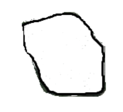
Behind Pierce College is Waughop Lake, which is used by many students for learning scientific concepts outside of a classroom. The approximate shape of the lake is shown below. If one of the science labs required students to estimate the surface area of the water, what strategy could they use for this irregularly shaped lake?
A possible strategy is to think that this lake is almost a rectangle, and so they could draw a rectangle over it. Since a formula is known for the area of a rectangle, and if we know that each arrow below is 200 meters, can the area of the lake be estimated?
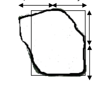
There are two important questions to consider. If this approach is taken, will the area of the lake exactly equal the area of the rectangle? Will it be close?
The answer to the first question is no, unless we happened to be extremely lucky with our drawing of the rectangle. The answer to the second question is yes it should be close. 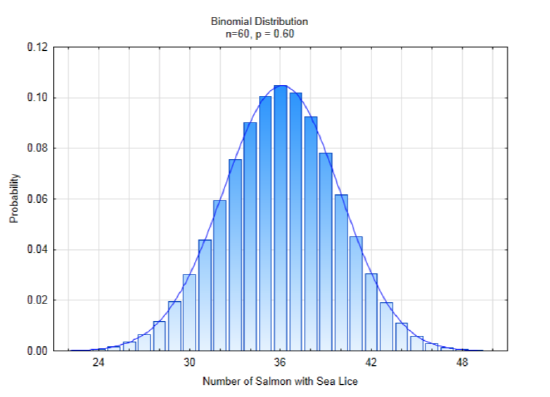
The concept of approximating an irregular shape with a shape for which the properties are know is the strategy we will use to find new ways of determining a p-value. To the right is the irregular shape of a binomial distribution if n = 60, p = 0.60. The smooth curve that is drawn over the top of the bars is called the normal distribution. It also goes by the names bell curve and Gaussian distribution.
The formula for the normal distribution is \(f(x, \mu, \sigma) = \dfrac{1}{\sigma \sqrt{2\pi}} e^{[\dfrac{1}{2} (\dfrac{x - \mu}{\sigma})^2]}\). It is not important that you know this formula. What is important is to notice the variables in it. Both πand e are constants with the values of 3.14159 and 2.71828 respectively. The x is the independent variable, which is found along the x-axis. The important variables to notice are μ and σ, the mean and standard deviation. The implication of these two variables is that they play an important role in defining this curve. The function can be shown as \(N(\mu,\sigma)\).
The binomial distribution is a discrete distribution whereas the normal distribution is a continuous distribution. It is known as a density function.
A normal distribution is contrasted with skewed distributions below.
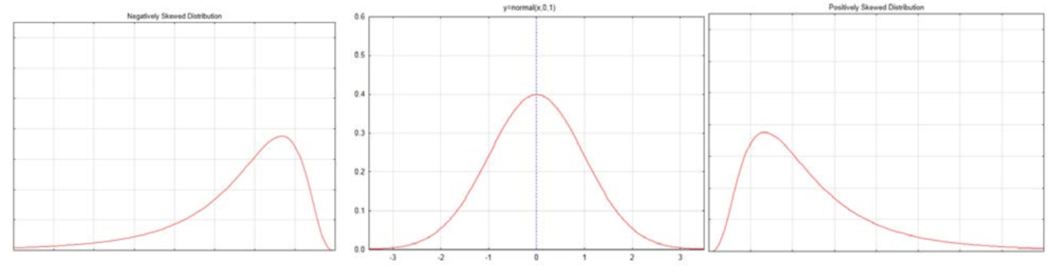
A negatively skewed distribution, such as is shown on the left, has some values that are very low causing the curve to be stretched to the left. These low values would cause the mean to be less than the median for the distribution. The positively skewed distribution, such as is shown on the right, has some values that are very high, causing the curve to be stretched to the right. These high values would cause the mean to be greater than the median for the distribution. The normal curve in the middle is symmetrical. The mean, median and mode are all in the middle. The mode is the high point of the curve.
The normal curve is called a density function, in contrast to the binomial distribution, which is a probability mass function. The space under the curve is called the area under the curve. The area is synonymous with the probability. The area under the entire curve, corresponding to the probability of selecting a value from anywhere in the distribution is 1. This curve never touches the x-axis, in spite of the fact that it looks like it does. Our ultimate objective with the nor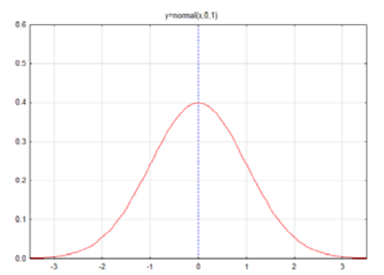 mal curve is to find the area in the tail, which corresponds with finding the p-value.
We will start to think about the area (probability) under the curve by looking at the standard normal curve. The standard normal curve has a mean of 0 and a standard deviation of 1 and is shown as a function N(0,1). Notice that the x-axis of the curve is numbered with –3, -2, -1, 0, 1, 2, 3. These numbers are called z scores. They represent the number of standard deviations x is from the mean, which is in the middle of the curve.
Does it seem reasonable that half of the curve is to the left of the mean and half the curve is to the right? We can label each side with this value, which is interpreted as both an area and a probability that a value would exist in that area.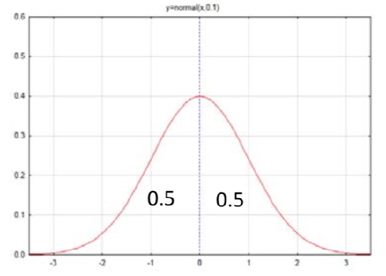
Thinking about the area under the normal distribution is not as easy as thinking about the area under a uniform distribution. For example, we could create a uniform distribution for the outcome of an experiment in which one die is rolled. The probability of rolling any number is 1/6. Therefore the uniform distribution would look like this.
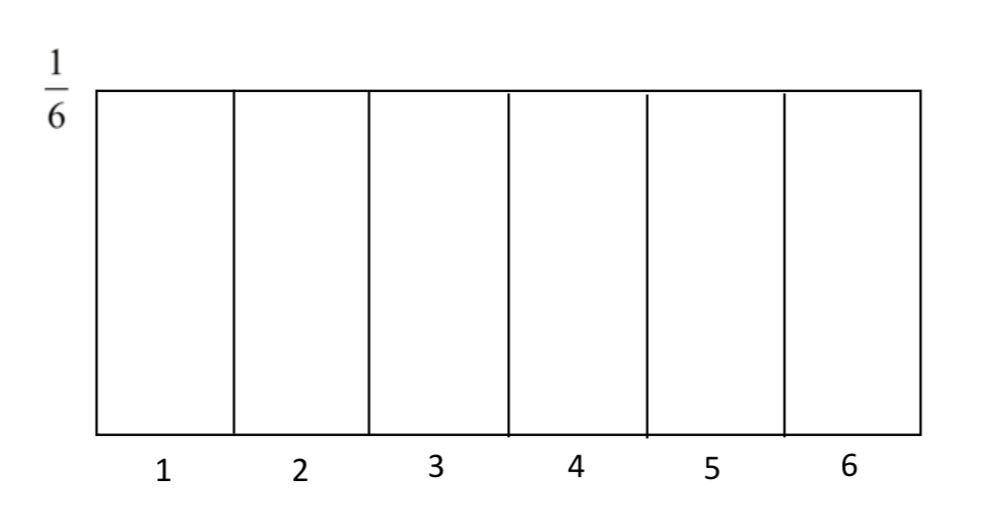
The area on this distribution can be found by multiplying the length by the width (height). Thus, to find the probability of getting a 5 or higher, we consider the length to be 2 and the width to be 1/6 so that \(2 \times (\dfrac{1}{6} = \dfrac{1}{3}\). That is, there is a probability of 1/3 that a 5 or 6 would be rolled on the die.
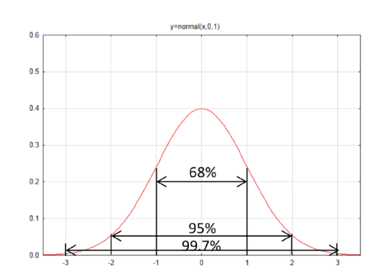
But a normal distribution is not as familiar as a rectangle, for which the area is easier to find. The Empirical Rule is an approximation of the areas for different sections of the normal curve; 68% of the curve is within one standard deviation of the mean, 95% of the curve is within two standard deviations of the mean, and 99.7% of the curve is within three standard deviations of the mean.
To find the area under a normal distribution was originally done using a technique called integration, which is taught in Calculus. However, these areas have already been found for the standard normal distribution N(0,1) and are provided in a table on the next page. The tables will always provide the area to the left. The area to the right is the complement of the area to the left, so to find the area to the right, subtract the area to the left from 1. A few examples should help clarify this.
Example 3. Find the areas to the left and right of z = -1.96.
Since the z value is less than 0, use the first of the two tables. Find the row with – 1.9 in the left column and find the column with the 0.06 in the top row. The intersection of those rows and columns gives the area to the left, designated as \(A_L\) as 0.0250. The area to the right, designated as \(A_R = 1 – 0.0250 = 0.9750\).
| Z | 0.09 | 0.08 | 0.07 | 0.06 | 0.05 | 0.04 | 0.03 | 0.02 | 0.01 | 0.00 |
| -1.9 | 0.0233 | 0.0239 | 0.0244 | 0.0250 | 0.0256 | 0.0262 | 0.0268 | 0.0274 | 0.0281 | 0.0287 |
Example 4. Find the areas to the left and right of z = 0.57.
Since the z value is greater than 0, use the second of the two tables. Find the row with 0.5 in the left column and find the column with 0.07 in the top row. The intersection of those rows and columns gives \(A_L = 0.7157\), therefore \(A_R = 1 – 0.7157 = 0.2843\).
Standard Normal Distribution – N(0,1)
Area to the left when \(z \le 0\)
| Z | 0.09 | 0.08 | 0.07 | 0.06 | 0.05 | 0.04 | 0.03 | 0.02 | 0.01 | 0.00 |
| -3.5 | 0.0002 | 0.0002 | 0.0002 | 0.0002 | 0.0002 | 0.0002 | 0.0002 | 0.0002 | 0.0002 | 0.0002 |
| -3.4 | 0.0002 | 0.0003 | 0.0003 | 0.0003 | 0.0003 | 0.0003 | 0.0003 | 0.0003 | 0.0003 | 0.0003 |
| -3.3 | 0.0003 | 0.0004 | 0.0004 | 0.0004 | 0.0004 | 0.0004 | 0.0004 | 0.0005 | 0.0005 | 0.0005 |
| -3.2 | 0.0005 | 0.0005 | 0.0005 | 0.0006 | 0.0006 | 0.0006 | 0.0006 | 0.0006 | 0.0007 | 0.0007 |
| -3.1 | 0.0007 | 0.0007 | 0.0008 | 0.0008 | 0.0008 | 0.0008 | 0.0009 | 0.0009 | 0.0009 | 0.0010 |
| -3.0 | 0.0010 | 0.0010 | 0.0011 | 0.0011 | 0.0011 | 0.0012 | 0.0012 | 0.0013 | 0.0013 | 0.0013 |
| -2.9 | 0.0014 | 0.0014 | 0.0015 | 0.0015 | 0.0016 | 0.0016 | 0.0017 | 0.0018 | 0.0018 | 0.0019 |
| -2.8 | 0.0019 | 0.0020 | 0.0021 | 0.0021 | 0.0022 | 0.0023 | 0.0023 | 0.0024 | 0.0025 | 0.0026 |
| -2.7 | 0.0026 | 0.0027 | 0.0028 | 0.0029 | 0.0030 | 0.0031 | 0.0032 | 0.0033 | 0.0034 | 0.0035 |
| -2.6 | 0.0036 | 0.0037 | 0.0038 | 0.0039 | 0.0040 | 0.0041 | 0.0043 | 0.0044 | 0.0045 | 0.0047 |
| -2.5 | 0.0048 | 0.0049 | 0.0051 | 0.0052 | 0.0054 | 0.0055 | 0.0057 | 0.0059 | 0.0060 | 0.0062 |
| -2.4 | 0.0064 | 0.0066 | 0.0068 | 0.0069 | 0.0071 | 0.0073 | 0.0075 | 0.0078 | 0.0080 | 0.0082 |
| -2.3 | 0.0084 | 0.0087 | 0.0089 | 0.0091 | 0.0094 | 0.0096 | 0.0099 | 0.0102 | 0.0104 | 0.0107 |
| -2.2 | 0.0110 | 0.0113 | 0.0116 | 0.0119 | 0.0122 | 0.0125 | 0.0129 | 0.0132 | 0.0136 | 0.0139 |
| -2.1 | 0.0143 | 0.0146 | 0.0150 | 0.0154 | 0.0158 | 0.0162 | 0.0166 | 0.0170 | 0.0174 | 0.0179 |
| -2.0 | 0.0183 | 0.0188 | 0.0192 | 0.0197 | 0.0202 | 0.0207 | 0.0212 | 0.0217 | 0.0222 | 0.0228 |
| -1.9 | 0.0233 | 0.0239 | 0.0244 | 0.0250 | 0.0256 | 0.0262 | 0.0268 | 0.0274 | 0.0281 | 0.0287 |
| -1.8 | 0.0294 | 0.0301 | 0.0307 | 0.0314 | 0.0322 | 0.0329 | 0.0336 | 0.0344 | 0.0351 | 0.0359 |
| -1.7 | 0.0367 | 0.0375 | 0.0384 | 0.0392 | 0.0401 | 0.0409 | 0.0418 | 0.0427 | 0.0436 | 0.0446 |
| -1.6 | 0.0455 | 0.0465 | 0.0475 | 0.0485 | 0.0495 | 0.0505 | 0.0516 | 0.0526 | 0.0537 | 0.0446 |
| -1.5 | 0.0559 | 0.0571 | 0.0582 | 0.0594 | 0.0606 | 0.0618 | 0.0630 | 0.0643 | 0.0655 | 0.0668 |
| -1.4 | 0.0681 | 0.0694 | 0.0708 | 0.0721 | 0.0735 | 0.0749 | 0.0764 | 0.0778 | 0.0793 | 0.0808 |
| -1.3 | 0.0823 | 0.0838 | 0.0853 | 0.0869 | 0.0885 | 0.0901 | 0.0918 | 0.0934 | 0.0951 | 0.0968 |
| -1.2 | 0.0985 | 0.1003 | 0.1020 | 0.1038 | 0.1056 | 0.1075 | 0.1093 | 0.1112 | 0.1131 | 0.1151 |
| -1.1 | 0.1170 | 0.1190 | 0.1210 | 0.1230 | 0.1251 | 0.1271 | 0.1292 | 0.1314 | 0.1334 | 0.1357 |
| -1.0 | 0.1379 | 0.1401 | 0.1423 | 0.1446 | 0.1469 | 0.1492 | 0.1515 | 0.1539 | 0.1562 | 0.1587 |
| -0.9 | 0.1611 | 0.1635 | 0.1660 | 0.1685 | 0.1711 | 0.1736 | 0.1762 | 0.1788 | 0.1814 | 0.1841 |
| -0.8 | 0.1867 | 0.1894 | 0.1922 | 0.1949 | 0.1977 | 0.2005 | 0.2033 | 0.2061 | 0.2090 | 0.2119 |
| -0.7 | 0.2148 | 0.2177 | 0.2206 | 0.2236 | 0.2266 | 0.2296 | 0.2327 | 0.2358 | 0.2389 | 0.2420 |
| -0.6 | 0.2451 | 0.2483 | 0.2514 | 0.2546 | 0.2578 | 0.2611 | 0.2643 | 0.2676 | 0.2709 | 0.2743 |
| -0.5 | 0.2776 | 0.2810 | 0.2843 | 0.2877 | 0.2912 | 0.2946 | 0.2981 | 0.3015 | 0.3050 | 0.3085 |
| -0.4 | 0.3121 | 0.3156 | 0.3192 | 0.3228 | 0.3264 | 0.3300 | 0.3336 | 0.3372 | 0.3409 | 0.3446 |
| -0.3 | 0.3483 | 0.3520 | 0.2557 | 0.3594 | 0.3632 | 0.3669 | 0.3707 | 0.3745 | 0.3783 | 0.3821 |
| -0.2 | 0.4247 | 0.4286 | 0.4325 | 0.4364 | 0.4404 | 0.4443 | 0.4483 | 0.4522 | 0.4562 | 0.4602 |
| 0.0 | 0.4641 | 0.4681 | 0.4721 | 0.4761 | 0.4801 | 0.4840 | 0.4880 | 0.4920 | 0.4960 | 0.5000 |
Standard Normal Distribution – N(0,1)
Area to the left when \(z \ge 0\)
| Z | 0.00 | 0.01 | 0.02 | 0.03 | 0.04 | 0.05 | 0.06 | 0.07 | 0.08 | 0.09 |
| 0.0 | 0.5000 | 0.5040 | 0.5080 | 0.5120 | 0.5160 | 0.5199 | 0.5239 | 0.5279 | 0.5319 | 0.5359 |
| 0.1 | 0.5398 | 0.5438 | 0.5478 | 0.5517 | 0.5557 | 0.5596 | 0.5636 | 0.5675 | 0.5714 | 0.5753 |
| 0.2 | 0.5793 | 0.5832 | 0.5871 | 0.5910 | 0.5948 | 0.5987 | 0.6026 | 0.6064 | 0.6103 | 0.6141 |
| 0.3 | 0.6179 | 0.6217 | 0.6255 | 0.6293 | 0.6331 | 0.6368 | 0.6406 | 0.6443 | 0.6480 | 0.6517 |
| 0.4 | 0.6554 | 0.6591 | 0.6628 | 0.6664 | 0.6700 | 0.6736 | 0.6772 | 0.6808 | 0.6844 | 0.6879 |
| 0.5 | 0.6915 | 0.6950 | 0.6985 | 0.7019 | 0.7054 | 0.7088 | 0.7123 | 0.7157 | 0.7190 | 0.7224 |
| 0.6 | 0.7257 | 0.7291 | 0.7324 | 0.7357 | 0.7389 | 0.7422 | 0.7454 | 0.7486 | 0.7517 | 0.7549 |
| 0.7 | 0.7580 | 0.7611 | 0.7642 | 0.7673 | 0.7704 | 0.7734 | 0.7764 | 0.7794 | 0.7823 | 0.7852 |
| 0.8 | 0.7881 | 0.7910 | 0.7939 | 0.7967 | 0.7995 | 0.8023 | 0.8051 | 0.8078 | 0.8106 | 0.8133 |
| 0.9 | 0.8159 | 0.8186 | 0.8212 | 0.8238 | 0.8264 | 0.8289 | 0.8315 | 0.8340 | 0.8365 | 0.8389 |
| 1.0 | 0.8413 | 0.8438 | 0.8461 | 0.8485 | 0.8508 | 0.8531 | 0.8554 | 0.8577 | 0.8599 | 0.8621 |
| 1.1 | 0.8643 | 0.8665 | 0.8686 | 0.8708 | 0.8729 | 0.8749 | 0.8770 | 0.8790 | 0.8810 | 0.8830 |
| 1.2 | 0.8849 | 0.8869 | 0.8888 | 0.8907 | 0.8925 | 0.8944 | 0.8962 | 0.8980 | 0.8997 | 0.9015 |
| 1.3 | 0.9032 | 0.9049 | 0.9066 | 0.9082 | 0.9099 | 0.9115 | 0.9131 | 0.9147 | 0.9162 | 0.9177 |
| 1.4 | 0.9192 | 0.9207 | 0.9222 | 0.9236 | 0.9251 | 0.9265 | 0.9279 | 0.9292 | 0.9306 | 0.9319 |
| 1.5 | 0.9332 | 0.9345 | 0.9357 | 0.9370 | 0.9382 | 0.9394 | 0.9406 | 0.9418 | 0.9429 | 0.9441 |
| 1.6 | 0.9452 | 0.9463 | 0.9474 | 0.9484 | 0.9495 | 0.9505 | 0.9515 | 0.9525 | 0.9535 | 0.9545 |
| 1.7 | 0.9554 | 0.9564 | 0.9573 | 0.9582 | 0.9591 | 0.9599 | 0.9608 | 0.9616 | 0.9625 | 0.9633 |
| 1.8 | 0.9641 | 0.9649 | 0.9656 | 0.9664 | 0.9671 | 0.9678 | 0.9686 | 0.9693 | 0.9699 | 0.9706 |
| 1.9 | 0.9713 | 0.9719 | 0.9726 | 0.9732 | 0.9738 | 0.9744 | 0.9750 | 0.9756 | 0.9761 | 0.9767 |
| 2.0 | 0.9772 | 0.9778 | 0.9783 | 0.9788 | 0.9793 | 0.9798 | 0.9803 | 0.9808 | 0.9812 | 0.9817 |
| 2.1 | 0.9821 | 0.9826 | 0.9830 | 0.9834 | 0.9838 | 0.9842 | 0.9846 | 0.9850 | 0.9854 | 0.9857 |
| 2.2 | 0.9861 | 0.9864 | 0.9868 | 0.9871 | 0.9875 | 0.9878 | 0.9881 | 0.9884 | 0.9887 | 0.9890 |
| 2.3 | 0.9893 | 0.9896 | 0.9898 | 0.9901 | 0.9904 | 0.9906 | 0.9909 | 0.9911 | 0.9913 | 0.9916 |
| 2.4 | 0.9918 | 0.9920 | 0.9922 | 0.9925 | 0.9927 | 0.9929 | 0.9931 | 0.9932 | 0.9934 | 0.9936 |
| 2.5 | 0.9938 | 0.9940 | 0.9941 | 0.9943 | 0.9945 | 0.9946 | 0.9948 | 0.9949 | 0.9951 | 0.9952 |
| 2.6 | 0.9953 | 0.9955 | 0.9956 | 0.9957 | 0.9959 | 0.9960 | 0.9961 | 0.9962 | 0.9963 | 0.9964 |
| 2.7 | 0.9965 | 0.9966 | 0.9967 | 0.9968 | 0.9969 | 0.9970 | 0.9971 | 0.9972 | 0.9973 | 0.9974 |
| 2.8 | 0.9974 | 0.9975 | 0.9976 | 0.9977 | 0.9977 | 0.9978 | 0.9979 | 0.9979 | 0.9980 | 0.9981 |
| 2.9 | 0.9981 | 0.9982 | 0.9982 | 0.9983 | 0.9984 | 0.9984 | 0.9985 | 0.9985 | 0.9986 | 0.9986 |
| 3.0 | 0.9987 | 0.9987 | 0.9987 | 0.9988 | 0.9988 | 0.9989 | 0.9989 | 0.9989 | 0.9990 | 0.9990 |
| 3.1 | 0.9990 | 0.9991 | 0.9991 | 0.9991 | 0.9992 | 0.9992 | 0.9992 | 0.9992 | 0.9993 | 0.9993 |
| 3.2 | 0.9993 | 0.9993 | 0.9994 | 0.9994 | 0.9994 | 0.9994 | 0.9994 | 0.9995 | 0.9995 | 0.9995 |
| 3.3 | 0.9995 | 0.9995 | 0..9995 | 0.9996 | 0.9996 | 0.9996 | 0.9996 | 0.9996 | 0.9996 | 0.9997 |
| 3.4 | 0.9997 | 0.9997 | 0.9997 | 0.9997 | 0.9997 | 0.9997 | 0.9997 | 0.9997 | 0.9997 | 0.9998 |
Since it is very unlikely that we will encounter authentic populations that are normally distributed with a mean of zero and a standard deviation of one, then of what use is this? The answer to this question has two parts. The first part is to answer the question about which useful populations are normally distributed. The second part is to determine how these tables can be used by other distributions with different means and standard deviations.
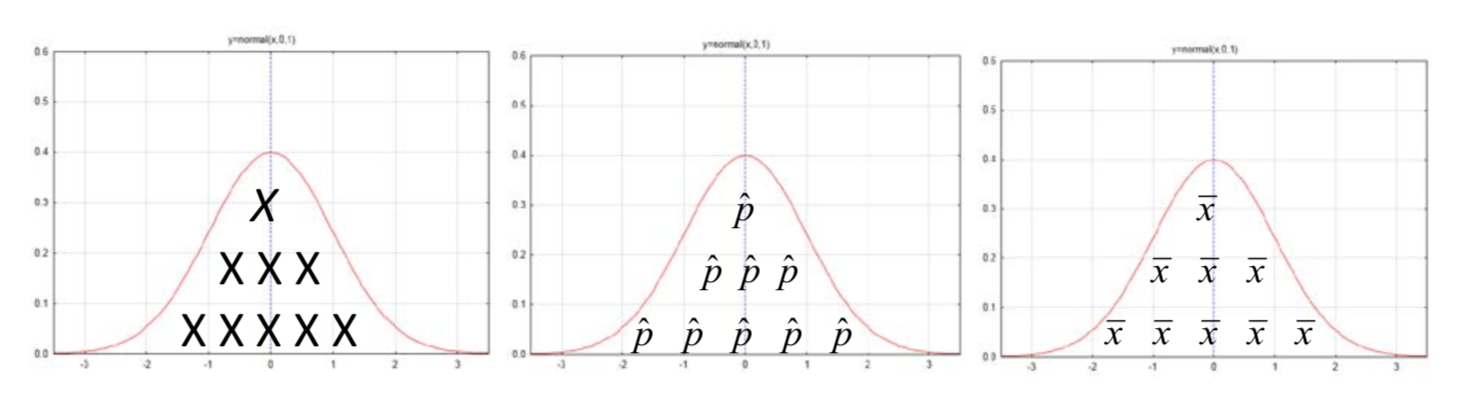
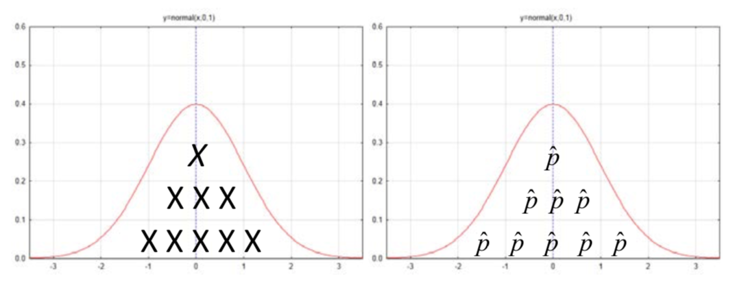
You have already seen that the normal curve fits very nicely over the binomial distribution. In chapters one and two you also saw distributions of sample proportions and sample means that look normally distributed. Therefore, the primary use of the normal distribution is to find probabilities when it is used to model other distributions such as the binomial distribution or the sampling distributions of \(\hat{p}\) or \(\bar{x}\). The following illustrate the elements of the distributions being modeled by the curve.
Now that some of the distributions that can be modeled with a normal curve have been established, we can address the second question, which is how to make use of the tables for the standard normal curve. Probabilities and more specifically p-values, can only be found after we have our sample results. Those sample results are part of a distribution of possible results that are approximately normally distributed. By determining the number of standard deviations our sample results are from the mean of the population, we can use the standard normal distribution tables to find the p-value. The transformation of sample results into standard deviations from the mean makes use of the z formula.
The z score is the number of standard deviations a value is from the mean. By subtracting the value from the mean and dividing by the standard deviation, we calculate the number of standard deviations. The formula is
\[z = \dfrac{x - \mu}{\sigma}\]
This is the basic formula upon which many others will be built.
Example 5
Suppose the mean number of successes in a sample of 100 is 20 and the standard deviation is 4. Sketch and label a normal curve and find the area in the left tail for the number 13.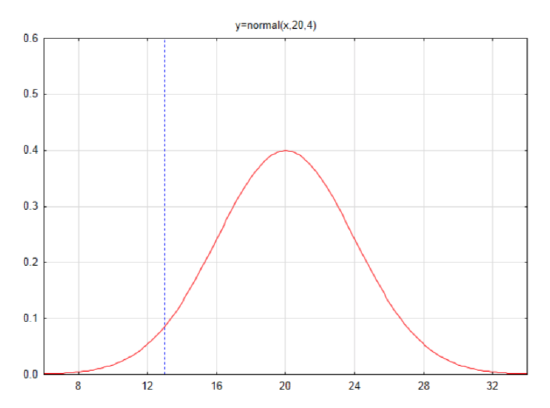
First find the z score: \(z = \dfrac{x - \mu}{\sigma}\)
\(z = \dfrac{13 - 20}{4} = -1.75\)
Find the area to the left in the table
\(A_L = 0.0401\)
Example 6
If the mean is 30 and the standard deviation is 5, then sketch and label a normal curve and find the area in the right tail for the number 44.1.
First find the z score: \(z = \dfrac{x - \mu}{\sigma}\)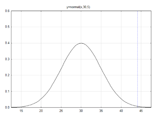
\(z = \dfrac{44.1 - 30}{5} = 2.82\)
Find the area to the left in the table
\(A_L = 0.9976\)
Use this to find the area to the right by subtracting from 1.
\(A_R = 0.0024\)
Return to Step 6: Apply this concept of probability to the hypothesis about the responsibility for a self-driving car in an accident.
Remember that the hypotheses for the autonomous car problem are: \(H_0: p = 0.60\), \(H_1: p > 0.60\). In the original problem, the researcher found that 4 out of 6 people thought the owner was responsible. Which hypothesis does this data support if the level of significance is 0.10?
This hypothesis test will be done using a method called the Normal Approximation to the Binomial Distribution.
The first step is to find the mean and standard deviation of the binomial distribution (which was done earlier but is now repeated):
\(\mu = np = 6(0.6) = 3.6\)
\(\sigma = \sqrt{npq} = \sqrt{6(0.6)(0.4)} = 1.2\)
Draw and label a normal curve with a mean of 3.6 and a standard deviation of 1.2.
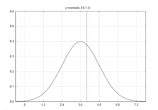
Find the z score if the data is 4.
\(z = \dfrac{x - \mu}{\sigma}\) \(z = \dfrac{4 - 3.6}{1.2} = 0.33\)
From the table, the area to the left is \(A_L = 0.6255\). Since the direction of the extreme is to the right, subtract the area to the left from 1 to get \(A_R = 0.3745\). This is the p-value.
This p-value can also be found with the calculator (\(2^{\text{nd}}\) Distr #2: normalcdf(low, high, \(\mu\), \(\sigma\))) shown as normalcdf(4, 1E99, 3.6,1.2)=0.3694.
Since this value is greater than the level of significance, if the calculator generated p-value is used, the conclusion will be written as: At the 0.10 level of significance, the proportion of people who think the owner is responsible is not significantly more than 0.60 (z = 0.33, p = 0.3694, n = 6).
Let us now take a moment to compare the p-value from the Normal Approximation to the Binomial Distribution (0.3694) to the exact p-value found using the Binomial Distribution (0.5443). While these p- values are not very close to each other, the conclusion that is drawn is the same. The reason they are not very close is because a sample size of 6 is very small and the normal approximation is not very good with a small sample size.
Test the hypothesis again if the researcher finds that 400 out of 600 of the people believe the owner is responsible for accidents.
\(\mu = np = 600(0.6) = 360\) This indicates that if lots of samples of 600 people were sampled the average number of people who think the owner is responsible would be 360.
\(\sigma = \sqrt{npq} = \sqrt{600(0.6)(0.4)} = 12\)
Draw a label a curve with a mean of 360 and a standard deviation of 12.
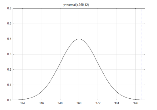
Find the z score if the data is 400.
\(z = \dfrac{x - \mu}{\sigma}\) \(z = \dfrac{400 - 360}{12} = 3.33\)
Using the table, the area to the left is \(A_L = 0.9996\). Since the direction of the extreme is to the right, subtract the area to the left from 1 to get \(A_R = 0.0004\). More precisely, it is 0.000430.
This time when the results of the Normal Approximation to the Binomial Distribution (0.000430) are compared to the results of the binomial distribution (0.000443), they are very close. This is because the sample size is larger.
In general, if \(np \ge 5\) and \(nq \ge 5\), then the normal approximation makes a good, but not perfect estimate for the binomial distribution. When a sample of size 6 was used, \(np = 3.6\) which is less than 5. Also, \(nq = 6(0.4) = 2.4\), which is less than 5, too. Therefore, using the normal approximation for samples that small is not a good strategy.
Step 7 – Find the approximate p-value using the Sampling Distribution of Sample Proportions
Up to this point the discussion has been about the number of people. When sampling that produces categorical data is done, these numbers or counts can also be represented as proportions by dividing the number of successes by the sample size. Thus, instead of the researcher saying that 4 out of 6 people believe the owner is responsible, the researcher could say that 66.7% of the people believe the owner is responsible. This leads to the concept of looking at proportions rather than counts which means that instead of the distribution being made up of the number of successes, represented by x, it is made up of the sample proportion of successes represented by \(\hat{p}\).
Digression 7 – Sampling Distribution of Sample Proportions
Since the binomial distribution contains all possible counts of the number of successes and it is approximately normally distributed and since all counts can be converted to proportions by dividing by the sample size, then the distribution of \(\hat{p}\) is also approximately normally distributed. This distribution has a mean and standard deviation that can be found by dividing the mean and standard deviation of the binomial distribution by the sample size n.
The mean of all the sample proportions is the mean number of successes divided by n.
\(\mu_{\hat{p}} = \dfrac{\mu}{n} = \dfrac{np}{n} = p\) This indicates that the mean of all possible sample proportions equals the true proportion for the population.
\[\mu_{\hat{p}} = p\]
The standard deviation of all the sample proportions is the standard deviation of the number of successes divided by n.
\(\sigma_{\hat{p}} = \dfrac{\sigma}{n} = \sqrt{\dfrac{npq}{n^2}} = \sqrt{\dfrac{pq}{n}}\ or\ \sqrt{\dfrac{p(1- p)}{n}}\)
\[\sigma_{\hat{p}} = \sqrt{\dfrac{pq}{n}}\ \ \ \ or \ \ \ \ \sigma_{\hat{p}} = \sqrt{\dfrac{p(1- p)}{n}}\]
The basic z formula \(z = \dfrac{x − \mu}{\sigma}\) can now be rewritten knowing that in a distribution of sample proportions, the results of the sample that have formerly been represented with \(X\) can now be represented with \(\hat{p}\). The mean, \(\mu\) can now be represented with \(p\), since \(\mu_{\hat{p}} = p\) and the standard deviation \(\sigma\) can now be represented with \(\sqrt{\dfrac{p(1- p)}{n}}\) since \(\sigma_{\hat{p}} = \sqrt{\dfrac{p(1- p)}{n}}\). Therefore, for the sampling distribution of sample proportions, the z formula \(z = \dfrac{x − \mu}{\sigma}\) becomes
\[z = \dfrac{\hat{p} - p}{\sqrt{\dfrac{p(1-p)}{n}}}.\]
Apply this concept of probability to the hypothesis about the responsibility for a self-driving car in an accident.
Remember that the hypotheses for the people who think the owner is responsible are: \(H_0: p = 0.60\), \(H_1: p > 0.60\). In the original problem, the researcher found that 4 out of 6 people think the owner is responsible. Which hypothesis does this data support if the level of significance is 0.10?
Since \(\mu_{\hat{p}} = p\) then the mean is 0.60 (from the null hypothesis).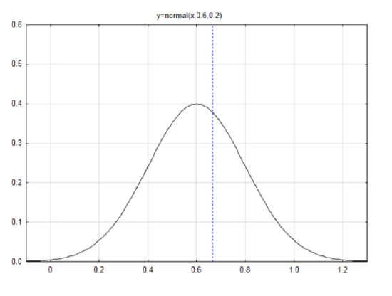
Since \(\sigma_{\hat{p}} = \sqrt{\dfrac{p(1-p)}{n}} = \sqrt{\dfrac{0.6(0.4)}{6}} = 0.2\) then the standard deviation is 0.2.
Draw a label a normal curve with a mean of 0.6 and a
standard deviation of 0.2.
If the data is 4, then the sample proportion,
\(\hat{p} = \dfrac{x}{n} = \dfrac{4}{6} = 0.6667\)
Find the z score if the data is 4.
\(z = \dfrac{\hat{p} - p}{\sqrt{\dfrac{p(1-p)}{n}}}\) \(z = \dfrac{0.6667 - 0.6}{0.2} = 0.33\)
The area to the left is \(A_L = 0.6304\). Since the direction of the extreme is to the right, subtract the area to the left from 1 to get \(A_R = 0.3696\).
Compare this result to the result found when using the Normal Approximation to the Binomial Distribution. Notice that both results are exactly the same. This should happen every time, provided there isn’t any rounding of numbers. The reason this has happened is because the number of successes can be represented as counts or proportions. The distributions are the same, although the x-axis is labeled differently. Divide the z scores for the normal approximation by the sample size 6 and you will get the z scores for the sampling distribution.
Test the hypothesis again if the researcher finds that 400 out of 600 of the people believe the owner is responsible.
Since \(\mu_{\hat{p}} = p\) then the mean is 0.60 (from the null hypothesis).
Since \(\sigma_{\hat{p}} = \sqrt{\dfrac{p(1-p)}{n}} = \sqrt{\dfrac{0.6(0.4)}{600}} = 0.02\) then the standard deviation is 0.02.
If the data is 400, then the sample proportion, \(\hat{p} = \dfrac{x}{n} = \dfrac{400}{600} = 0.66667\)
\(z = \dfrac{\hat{p} - p}{\sqrt{\dfrac{p(1-p)}{n}}}\) \(z = \dfrac{0.66667 - 0.6}{0.02} = 3.33\)
The area to the left is \(A_L = 0.9996\). Since the direction of the extreme is to the right, subtract the area to the left from 1 to get \(A_R = 0.0004\). More precisely, it is 0.000430.
Conclusion for testing hypotheses about categorical data.
By this time, many students are wondering why there are three methods and why the binomial distribution method isn’t the only one that is used since it produces an exact p-value. One justification of using the last method is comparing the results of surveys or other data. Imagine if one news organization reported their results of a survey as 670 out of 1020 were in favor while another organization reported they found 630 out of 980 were in favor. A comparison between these would be difficult without converting them to proportions, therefore, the third method, which uses proportions, is the method of choice. When the sample size is sufficiently large, there is not much difference between the methods. For smaller samples, it may be more appropriate to use the binomial distribution.
Making inferences using quantitative Data
The strategy for making inferences with quantitative data uses sampling distributions in the same way that they were used for making inferences about proportions. In that case, the normal distribution was used to model the distribution of sample proportions, pˆ . With quantitative data, we find the mean, therefore the normal distribution will be used to model the distribution of sample means, x .
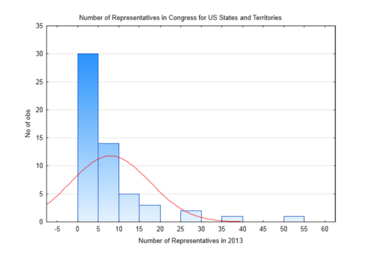
To demonstrate this, a small population will be used. This population consists of the 50 states of the United States plus the District of Columbia and the 5 US territories of American Samoa, Guam, Northern Mariana Islands, Puerto Rico and the Virgin Islands, each of which has one representative in Congress with limited voting authority. A histogram showing the distribution of the number of representatives in a state or territory is provided. On the graph is a normal distribution based on the mean of this population being 7.875 representatives and a standard deviation of 9.487. The distribution is positively skewed and cannot be modeled by the normal curve that is on the graph.
Be aware that in reality, the mean and standard deviation, which are parameters, are not known and so we would normally write hypotheses about them. However, for this demonstration, a small population with a known mean and standard deviation are necessary. With this, it is possible to illustrate what happens when repeated samples of the same size are drawn from this population, with replacement, and the means of each sample are found and becomes part of the distribution of sample means.
A sampling distribution of sample means (a distribution of x ) contains all possible sample means that in theory could be obtained if a random selection process was used, with replacement. The number of possible sample means can be found using the fundamental rule of counting. Draw a line to represent each state/territory that would be selected. On the line write the number of options, so that it would look like this:
| Options: | 56 | 56 | 56 | 56 | 56 |
| State: | 1 | 2 | 3 | 4... | n |
If our sample size is 40, then there are \(56^{40}\) possible samples that could be selected which is equal to \(8.46 \times 10^{69}\). That is a lot of possible samples. For this demonstration, only 10,000 samples of size 40 will be taken. The distribution of these sample means when this was done is shown in the histogram below.
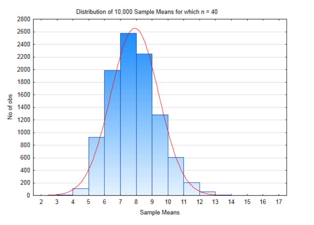
The mean of all these sample means is 7.8748 and the standard deviation is 1.502. Notice that the mean of all these sample means is almost exactly the same as the mean of the original population. Also notice that the standard deviation of all these sample means is much smaller than the standard deviation of the population. This is summarized in the table below.
| Population | Sampling Distribution | |
|---|---|---|
| Mean | 7.875 | 7.8748 |
| Standard Deviation | 9.487 | 1.502 |
The following graph has both the original data and the sample means on it. Notice how the two normal curves are centered at approximately the same place but the curve for the sample means is narrower. This shows that when samples of sufficient size are taken from any population, the means of those samples will be close to the means of the population.
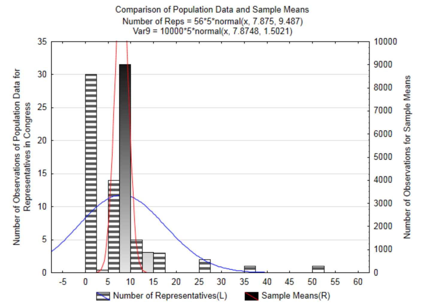
We are now ready to discuss the Central Limit Theorem. This theorem states that for any set of quantitative data with a mean μ and a standard deviation σ, the mean of all possible sample means will equal the mean of the population. The standard deviation of all the sample means, which is also called the standard error, will equal the standard deviation of the population divided by the square root of n. These are shown as:
\[\mu_{\bar{x}} = \mu\]
and
\[\sigma_{\bar{x}} = \dfrac{\sigma}{\sqrt{n}}.\]
It also says the distribution of sample means will be normal if the sample size is sufficiently large (generally considered to be 30 or more). If the original population is normally distributed, than the distribution of sample means will be normally distributed for any sample size.
Before doing an example, it will be important to see the effect of sample sizes. Compare the following 4 graphs that show the distribution of sample means for samples of size 40, 30, 20, and 10.
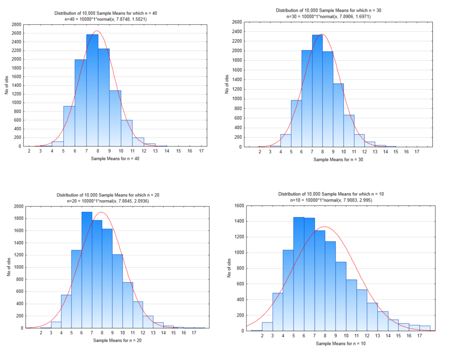
Notice how the distributions become more skewed as the sample size decreases. Notice also that the mean of the sample means are still approximately equal to the mean of the population but the standard deviations get larger as the sample size gets smaller. This implies there is more variation in sample means with small sample sizes than with large sample sizes.
| Population | \(n = 40\) | \(n = 30\) | \(n = 20\) | \(n = 10\) | |
|---|---|---|---|---|---|
| Mean | 7.875 | 7.8748 | 7.8906 | 7.8845 | 7.9083 |
| Standard Deviation | 9.487 | 1.5021 | 1.6971 | 2.0936 | 2.995 |
| Calculated Standard Deviation using \(\sigma_{\bar{x}} = \dfrac{\sigma}{\sqrt{n}}\) |
1.500 | 1.732 | 2.121 | 3.000 |
When making inferences about quantitative data, the basic \(z\) formula \(z = \dfrac{x − μ}{\sigma}\) can now be rewritten knowing that in a distribution of sample means, the results of the sample that have formerly been represented with \(x\) can now be represented with \(\bar{x}\). The mean, \(\mu\) will still be represented with \(\mu\), since \(\mu_{\bar{x}} = \mu\) and the standard deviation \(\sigma\) can now be represented with \(\dfrac{\sigma}{\sqrt{n}}\) since \(\sigma_{\bar{x}} = \dfrac{\sigma}{\sqrt{n}}\)
Therefore, for the sampling distribution of sample means, the \(z\) formula, \(z = \dfrac{x − μ}{\sigma}\) becomes
\[z = \dfrac{\bar{x} - \mu}{\dfrac{\sigma}{\sqrt{n}}}.\]
It is now time to use the central limit theorem to test a hypothesis.
Example 7
Example 7 Mercury in fish is not healthy and restrictions are placed on the amount of fish that should be eaten. Suppose a researcher wanted to know if the average concentration of methylmercury per kilogram of fish tissue was greater than the maximum recommended limit of 300 μg/kg. If the average concentration is greater than 300, the fisheries will be closed, otherwise it will remain open. Suppose also that the standard deviation for the population is \(\sigma = 50 \mu g/kg\). The researcher catches 36 fish. The sample mean concentration is 310.
The hypotheses to be tested are:
\(H_0: \mu = 300\)
\(H_1: \mu > 300\)
\(\alpha = 0.1\)
Since all the information that is needed is provided in the problem, the first step is to find the \(z\) score.
\(z = \dfrac{\bar{x} - \mu}{\dfrac{\sigma}{\sqrt{n}}} = \dfrac{310 - 300}{\dfrac{50}{\sqrt{36}}} = 1.2.\)
The next step is to look up 1.20 in the standard normal distribution tables. This gives an area to the left of \(A_L=0.8849\) and so the area to the right is \(A_R = 0.1151\). This is a p-value.
Since the p-value is greater than the level of significance, the conclusion is that the average concentration of methylmercury in the fish tissue is not significantly greater than 300 \(\mu\)g/kg (\(z\) = 1.20, \(p\) = 0.1151, \(n\) = 36). Therefore, the fisheries will not be closed to fishing
Example 8
According to one estimate, the average wait time for subsidized housing for homeless people is 35 months.(www.stcloudstate.edu/reslife/...Statistics.pdf viewed 9/13/13) Assume the distribution of times is normal and the standard deviation is 10 months. One city evaluates its current program and to see if it is effective and justifies continued funding. If the average wait time is less than 35 months, the program will continue. Otherwise, the program will be replaced with a different program.
The hypotheses to be tested are:
- \(H_0: \mu = 35\)
- \(H-1: \mu < 35\)
\(\alpha = 0.01\)
The wait time (in months) of twenty people who recently received subsidized housing is recorded below.
| 44 | 23 | 26 | 27 | 22 | 33 | 20 | 28 | 8 | 22 |
| 23 | 19 | 12 | 23 | 12 | 7 | 17 | 4 | 18 | 33 |
Since we are given the data, we must find the sample mean before finding the z score.
\(\bar{x} = 21.05\)
\(z = \dfrac{\bar{x} - \mu}{\dfrac{\sigma}{\sqrt{n}}} = \dfrac{21.05 - 35}{\dfrac{10}{\sqrt{20}}} = -6.24.\)
Because the direction of the extreme is to the left we find the area to the left on the standard normal distribution table. The lowest z score we find on that table is -3.49. The area to the left of -3.49 is 0.0002. Going even further to the left, the area will be less than that. Therefore, the p-value for this data is <0.0002. The amount of wait time before people receive subsidized housing with the current program is significantly less than 35 months (z = -6.24, p < 0.0002, n = 20). Based on the decision rule, the program is effective and will continue to be funded.