Causation

CO-1: Describe the roles biostatistics serves in the discipline of public health.

Video

Video: Causation (8:45)

Introduction

Learning Objectives

LO 1.6: Recognize the distinction between association and causation.

Learning Objectives

LO 1.7: Identify potential lurking variables for explaining an observed relationship.

So far we have discussed different ways in which data can be used to explore the relationship (or association) between two variables. To frame our discussion we followed the role-type classification table:

We have now completed learning how to explore the relationship in cases C→Q, C→C, and Q→Q. (As noted before, case Q→C will not be discussed in this course.)

When we explore the relationship between two variables, there is often a temptation to conclude from the observed relationship that changes in the explanatory variable cause changes in the response variable. In other words, you might be tempted to interpret the observed association as causation.

The purpose of this part of the course is to convince you that this kind of interpretation is often wrong! The motto of this section is one of the most fundamental principles of this course:

WORDS TO LIVE BY: Statistical analysis alone will never prove causation!

PRINCIPLE: Association does not imply causation!

Outside Reading: Cause & Effect (≈ 1700 words)

Let’s start by looking at the following example:

EXAMPLE: Fire Damage

The scatterplot below illustrates how the number of firefighters sent to fires (X) is related to the amount of damage caused by fires (Y) in a certain city.

The scatterplot clearly displays a fairly strong (slightly curved) positive relationship between the two variables. Would it, then, be reasonable to conclude that sending more firefighters to a fire causes more damage, or that the city should send fewer firefighters to a fire, in order to decrease the amount of damage done by the fire? Of course not! So what is going on here?

There is a third variable in the background — the seriousness of the fire — that is responsible for the observed relationship. More serious fires require more firefighters, and also cause more damage.

The following figure will help you visualize this situation:

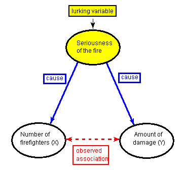
Here, the seriousness of the fire is a lurking variable. A lurking variable is a variable that is not among the explanatory or response variables in a study, but could substantially affect your interpretation of the relationship among those variables.

Here we have the following three relationships:

• Damage increases with the number of firefighters
• Number of firefighters increases with severity of fire
• Damage increases with the severity of fire
• Thus the increase in damage with the number of firefighters may be partially or fully explained by severity of fire.

In particular, as in our example, the lurking variable might have an effect on both the explanatory and the response variables. This common effect creates the observed association between the explanatory and response variables, even though there is no causal link between them. This possibility, that there might be a lurking variable (which we might not be thinking about) that is responsible for the observed relationship leads to our principle:

PRINCIPLE: Association does not imply causation!

The next example will illustrate another way in which a lurking variable might interfere and prevent us from reaching any causal conclusions.

EXAMPLE: SAT Test

For U.S. colleges and universities, a standard entrance examination is the SAT test. The side-by-side boxplots below provide evidence of a relationship between the student’s country of origin (the United States or another country) and the student’s SAT Math score.

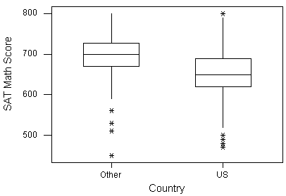
The distribution of international students’ scores is higher than that of U.S. students. The international students’ median score (about 700) exceeds the third quartile of U.S. students’ scores. Can we conclude that the country of origin is the cause of the difference in SAT Math scores, and that students in the United States are weaker at math than students in other countries?

No, not necessarily. While it might be true that U.S. students differ in math ability from other students — i.e. due to differences in educational systems — we can’t conclude that a student’s country of origin is the cause of the disparity. One important lurking variable that might explain the observed relationship is the educational level of the two populations taking the SAT Math test. In the United States, the SAT is a standard test, and therefore a broad cross-section of all U.S. students (in terms of educational level) take this test. Among all international students, on the other hand, only those who plan on coming to the U.S. to study, which is usually a more selected subgroup, take the test.

The following figure will help you visualize this explanation:

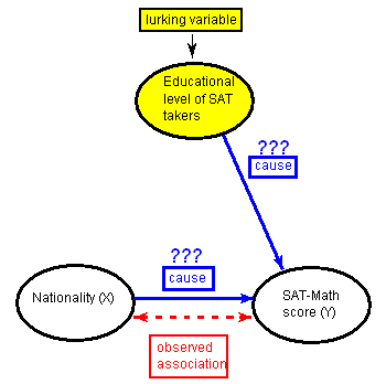
Here, the explanatory variable (X) may have a causal relationship with the response variable (Y), but the lurking variable might be a contributing factor as well, which makes it very hard to isolate the effect of the explanatory variable and prove that it has a causal link with the response variable. In this case, we say that the lurking variable is confounded with the explanatory variable, since their effects on the response variable cannot be distinguished from each other.

Note that in each of the above two examples, the lurking variable interacts differently with the variables studied. In example 1, the lurking variable has an effect on both the explanatory and the response variables, creating the illusion that there is a causal link between them. In example two, the lurking variable is confounded with the explanatory variable, making it hard to assess the isolated effect of the explanatory variable on the response variable.

The distinction between these two types of interactions is not as important as the fact that in either case, the observed association can be at least partially explained by the lurking variable. The most important message from these two examples is therefore: An observed association between two variables is not enough evidence that there is a causal relationship between them.

In other words …

PRINCIPLE: Association does not imply causation!

Learn By Doing: Causation

Simpson’s Paradox

Learning Objectives

LO 1.8: Recognize and explain the phenomenon of Simpson’s Paradox as it relates to interpreting the relationship between two variables.

So far, we have:

• discussed what lurking variables are,
• demonstrated different ways in which the lurking variables can interact with the two studied variables, and
• understood that the existence of a possible lurking variable is the main reason why we say that association does not imply causation.

As you recall, a lurking variable, by definition, is a variable that was not included in the study, but could have a substantial effect on our understanding of the relationship between the two studied variables.

What if we did include a lurking variable in our study? What kind of effect could that have on our understanding of the relationship? These are the questions we are going to discuss next.

Let’s start with an example:

EXAMPLE: Hospital Death Rates

Background: A government study collected data on the death rates in nearly 6,000 hospitals in the United States. These results were then challenged by researchers, who said that the federal analyses failed to take into account the variation among hospitals in the severity of patients’ illnesses when they were hospitalized. As a result, said the researchers, some hospitals were treated unfairly in the findings, which named hospitals with higher-than-expected death rates. What the researchers meant is that when the federal government explored the relationship between the two variables — hospital and death rate — it also should have included in the study (or taken into account) the lurking variable — severity of illness.

We will use a simplified version of this study to illustrate the researchers’ claim, and see what the possible effect could be of including a lurking variable in a study. (Reference: Moore and McCabe (2003). Introduction to the Practice of Statistics.)

Consider the following two-way table, which summarizes the data about the status of patients who were admitted to two hospitals in a certain city (Hospital A and Hospital B). Note that since the purpose of the study is to examine whether there is a “hospital effect” on patients’ status, “Hospital is the explanatory variable, and “Patient’s Status” is the response variable.

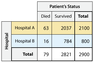
When we supplement the two-way table with the conditional percents within each hospital:

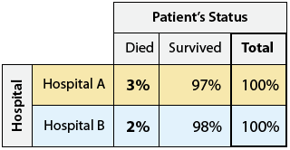
we find that Hospital A has a higher death rate (3%) than Hospital B (2%). Should we jump to the conclusion that a sick patient admitted to Hospital A is 50% more likely to die than if he/she were admitted to Hospital B? Not so fast …

Maybe Hospital A gets most of the severe cases, and that explains why it has a higher death rate. In order to explore this, we need to include (or account for) the lurking variable “severity of illness” in our analysis. To do this, we go back to the two-way table and split it up to look separately at patients who are severely ill, and patients who are not.

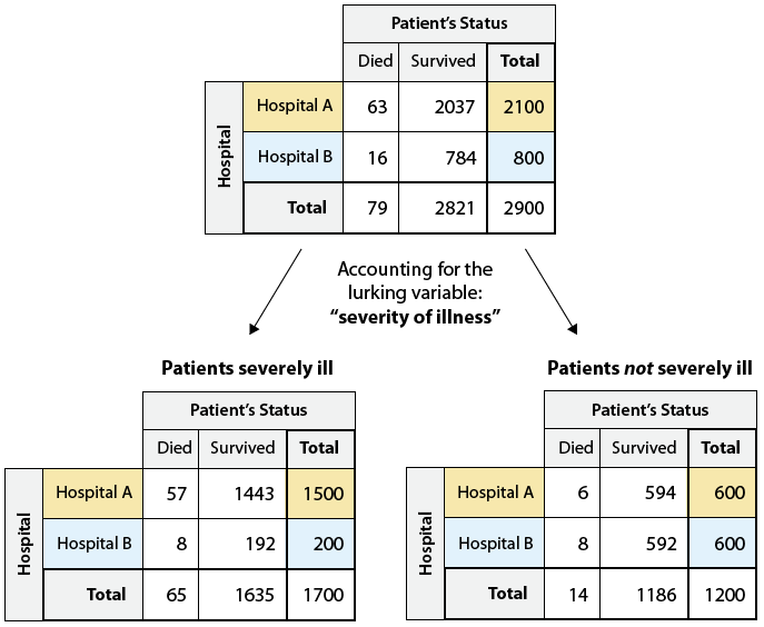
As we can see, Hospital A did admit many more severely ill patients than Hospital B (1,500 vs. 200). In fact, from the way the totals were split, we see that in Hospital A, severely ill patients were a much higher proportion of the patients — 1,500 out of a total of 2,100 patients. In contrast, only 200 out of 800 patients at Hospital B were severely ill. To better see the effect of including the lurking variable, we need to supplement each of the two new two-way tables with its conditional percentages:

Note that despite our earlier finding that overall Hospital A has a higher death rate (3% vs. 2%), when we take into account the lurking variable, we find that actually it is Hospital B that has the higher death rate both among the severely ill patients (4% vs. 3.8%) and among the not severely ill patients (1.3% vs. 1%). Thus, we see that adding a lurking variable can change the direction of an association.

Here we have the following three relationships:

• A greater percentage of hospital A’s patient’s died compared to hospital B.
• Patient’s who are severely ill are less likely to survive.
• Hospital A accepts more severely ill patients.
• In this case, after further careful analysis, we see that once we account for severity of illness, hospital A actually has a lower percentage of patient’s who died than hospital B in both groups of patients!

Whenever including a lurking variable causes us to rethink the direction of an association, this is called Simpson’s paradox.

The possibility that a lurking variable can have such a dramatic effect is another reason we must adhere to the principle:

PRINCIPLE: Association does not imply causation!

A Final Example – Gaining a Deeper Understaing of the Relationship

It is not always the case that including a lurking variable makes us rethink the direction of the association. In the next example we will see how including a lurking variable just helps us gain a deeper understanding of the observed relationship.

EXAMPLE: College Entrance Exams

As discussed earlier, in the United States, the SAT is a widely used college entrance examination, required by the most prestigious schools. In some states, a different college entrance examination is prevalent, the ACT.

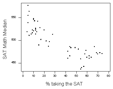
Note that:

• the explanatory variable is the percentage taking the SAT,
• the response variable is the median SAT Math score, and
• each data point on the scatterplot represents one of the states, so for example, in Illinois, in the year these data were collected, 16% of the students took the SAT Math, and their median score was 528.

Notice that there is a negative relationship between the percentage of students who take the SAT in a state, and the median SAT Math score in that state. What could the explanation behind this negative trend be? Why might having more people take the test be associated with lower scores?

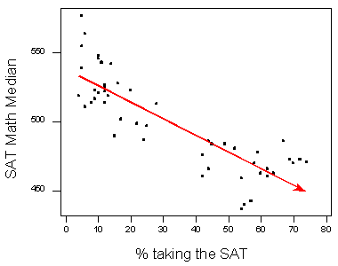
Note that another visible feature of the data is the presence of a gap in the middle of the scatterplot, which creates two distinct clusters in the data. This suggests that maybe there is a lurking variable that separates the states into these two clusters, and that including this lurking variable in the study (as we did, by creating this labeled scatterplot) will help us understand the negative trend.

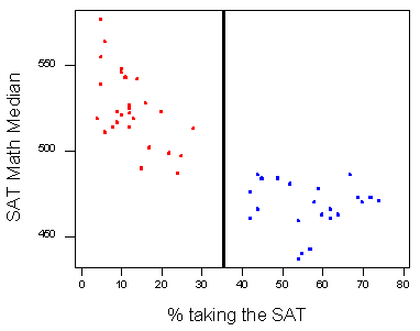
It turns out that indeed, the clusters represent two groups of states:

• The “blue group” on the right represents the states where the SAT is the test of choice for students and colleges.
• The “red group” on the left represents the states where the ACT college entrance examination is commonly used.

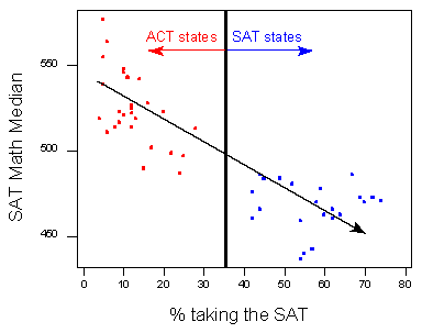
It makes sense then, that in the “ACT states” on the left, a smaller percentage of students take the SAT. Moreover, the students who do take the SAT in the ACT states are probably students who are applying to more prestigious national colleges, and therefore represent a more select group of students. This is the reason why we see high SAT Math scores in this group.

On the other hand, in the “SAT states” on the right, larger percentages of students take the test. These students represent a much broader cross-section of the population, and therefore we see lower (more average) SAT Math scores.

To summarize: In this case, including the lurking variable “ACT state” versus “SAT state” helped us better understand the observed negative relationship in our data.

Learn By Doing: Causation and Lurking Variables

Did I Get This?: Simpson’s Paradox

The last two examples showed us that including a lurking variable in our exploration may:

• lead us to rethink the direction of an association (as in the Hospital/Death Rate example) or,
• help us to gain a deeper understanding of the relationship between variables (as in the SAT/ACT example).

Let’s Summarize

• A lurking variable is a variable that was not included in your analysis, but that could substantially change your interpretation of the data if it were included.

• Because of the possibility of lurking variables, we adhere to the principle that association does not imply causation.

• Including a lurking variable in our exploration may:
  • help us to gain a deeper understanding of the relationship between variables, or
  • lead us to rethink the direction of an association (Simpson’s Paradox)

• Whenever including a lurking variable causes us to rethink the direction of an association, this is an instance of Simpson’s paradox.