Case C-C

CO-4: Distinguish among different measurement scales, choose the appropriate descriptive and inferential statistical methods based on these distinctions, and interpret the results.

Learning Objectives

LO 4.20: Classify a data analysis situation involving two variables according to the “role-type classification.”

Learning Objectives

LO 4.21: For a data analysis situation involving two variables, determine the appropriate graphical display(s) and/or numerical measures(s) that should be used to summarize the data.

Video

Video: Case C-C (10:34)

Related SAS Tutorials

• 6A – (3:07) Two-Way (Contingency) Tables – EDA

Related SPSS Tutorials

• 6A – (7:57) Two-Way (Contingency) Tables – EDA

Two Categorical Variables

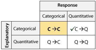
Recall the role-type classification table for framing our discussion about the relationship between two variables:

We are done with case C→Q, and will now move on to case C→C, where we examine the relationship between two categorical variables.

Earlier in the course, (when we discussed the distribution of a single categorical variable) we examined the data obtained when a random sample of 1,200 U.S. college students were asked about their body image (underweight, overweight, or about right). We are now returning to this example, to address the following question:

If we had separated our sample of 1,200 U.S. college students by gender and looked at males and females separately, would we have found a similar distribution across body-image categories? More specifically, are men and women just as likely to think their weight is about right? Among those students who do not think their weight is about right, is there a difference between the genders in feelings about body image?

Answering these questions requires us to examine the relationship between two categorical variables, gender and body image. Because the question of interest is whether there is a gender effect on body image,

• the explanatory variable is gender, and
• the response variable is body image.

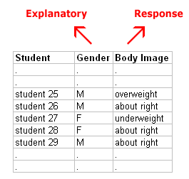
Here is what the raw data look like when we include the gender of each student:

Once again the raw data is a long list of 1,200 genders and responses, and thus not very useful in that form.

Contingency Tables

Learning Objectives

LO 4.22: Define and explain the process of creating a contingency table (two-way table).

To start our exploration of how body image is related to gender, we need an informative display that summarizes the data. In order to summarize the relationship between two categorical variables, we create a display called a two-way table or contingency table.

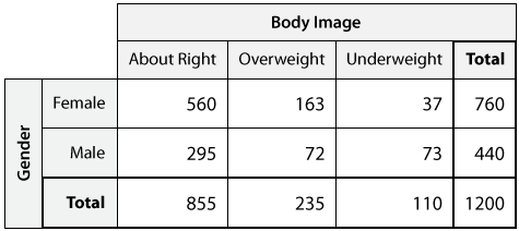
Here is the two-way table for our example:

The table has the possible genders in the rows, and the possible responses regarding body image in the columns. At each intersection between row and column, we put the counts for how many times that combination of gender and body image occurred in the data. We sum across the rows to fill in the Total column, and we sum across the columns to fill in the Total row.

Complete the following activities related to this data.

Learn By Doing: Case C-C

Comments:

Note that from the way the two-way table is constructed, the Total row or column is a summary of one of the two categorical variables, ignoring the other. In our example:

• The Total row gives the summary of the categorical variable body image:

• The Total column gives the summary of the categorical variable gender:(These are the same counts we found earlier in the course when we looked at the single categorical variable body image, and did not consider gender.)

Finding Conditional (Row and Column) Percents

Learning Objectives

LO 4.23: Given a contingency table (two-way table), interpret the information it reveals about the association between two categorical variables by calculating and comparing conditional percentages.

So far we have organized the raw data in a much more informative display — the two-way table:

Remember, though, that our primary goal is to explore how body image is related to gender. Exploring the relationship between two categorical variables (in this case body image and gender) amounts to comparing the distributions of the response variable (in this case body image) across the different values of the explanatory variable (in this case males and females):

Note that it doesn’t make sense to compare raw counts, because there are more females than males overall. So for example, it is not very informative to say “there are 560 females who responded ‘about right’ compared to only 295 males,” since the 560 females are out of a total of 760, and the 295 males are out of a total of only 440.

We need to supplement our display, the two-way table, with some numerical measures that will allow us to compare the distributions. These numerical measures are found by simply converting the counts to percents within (or restricted to) each value of the explanatory variable separately.

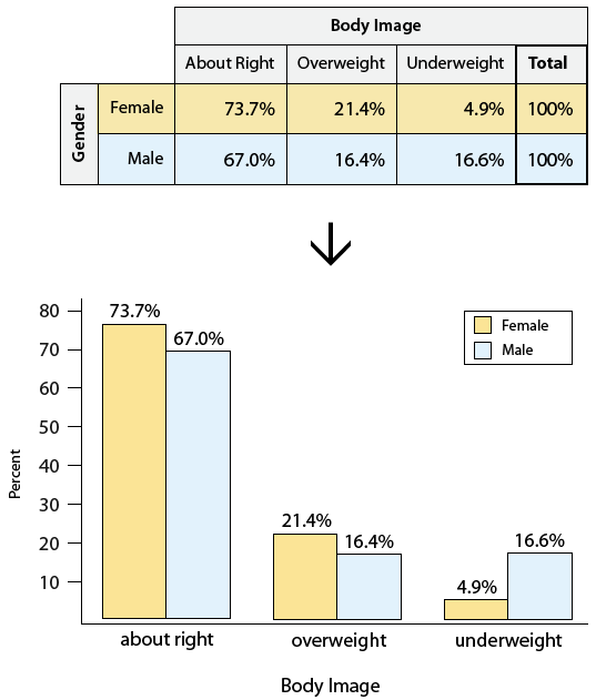
In our example: We look at each gender separately, and convert the counts to percents within that gender. Let’s start with females:

Note that each count is converted to percents by dividing by the total number of females, 760. These numerical measures are called conditional percents, since we find them by “conditioning” on one of the genders.

Now complete the following activities to calculate the row percentages for males.

Learn By Doing: Calculating Row Percentages

Comments:

• In our example, we chose to organize the data with the explanatory variable gender in rows and the response variable body image in columns, and thus our conditional percents were row percents, calculated within each row separately. Similarly, if the explanatory variable happens to sit in columns and the response variable in rows, our conditional percents will be column percents, calculated within each column separately. For an example, see the “Did I Get This?” exercises below.

• Another way to visualize the conditional percents, instead of a table, is the double bar chart. This display is quite common in newspapers.

Now that we have summarized the relationship between the categorical variables gender and body image, let’s go back and interpret the results in the context of the questions that we posed.

Learn By Doing: Interpretation in Case C-C

Learn By Doing: Case C-C (Software)

For additional practice complete the following activities.

Did I Get This?: Case C-C

Let’s Summarize

• The relationship between two categorical variables is summarized using:
  • Data display: two-way table, supplemented by
  • Numerical measures: conditional percentages.
• Conditional percentages are calculated for each value of the explanatory variable separately. They can be row percentages, if the explanatory variable “sits” in the rows, or column percentages, if the explanatory variable “sits” in the columns.
• When we try to understand the relationship between two categorical variables, we compare the distributions of the response variable for values of the explanatory variable. In particular, we look at how the pattern of conditional percentages differs between the values of the explanatory variable.