10.8: t Distribution

Learning Objectives

• State the difference between the shape of the \(t\) distribution and the normal distribution
• State how the difference between the shape of the \(t\) distribution and normal distribution is affected by the degrees of freedom
• Use a \(t\) table to find the value of \(t\) to use in a confidence interval
• Use the \(t\) calculator to find the value of \(t\) to use in a confidence interval

In the introduction to normal distributions it was shown that \(95\%\) of the area of a normal distribution is within \(1.96\) standard deviations of the mean. Therefore, if you randomly sampled a value from a normal distribution with a mean of \(100\), the probability it would be within \(1.96\sigma \) of \(100\) is \(0.95\). Similarly, if you sample \(N\) values from the population, the probability that the sample mean (\(M\)) will be within \(1.96\sigma _M\) of \(100\) is \(0.95\).

Now consider the case in which you have a normal distribution but you do not know the standard deviation. You sample \(N\) values and compute the sample mean (\(M\)) and estimate the standard error of the mean (\(\sigma _M\)) with \(s_M\). What is the probability that \(M\) will be within \(1.96 s_M\) of the population mean (\(\mu\))?

This is a difficult problem because there are two ways in which \(M\) could be more than \(1.96 s_M\) from \(\mu\):

1. \(M\) could, by chance, be either very high or very low and
2. \(s_M\) could, by chance, be very low.

Intuitively, it makes sense that the probability of being within \(1.96\) standard errors of the mean should be smaller than in the case when the standard deviation is known (and cannot be underestimated). But exactly how much smaller? Fortunately, the way to work out this type of problem was solved in the early \(20^{th}\) century by W. S. Gosset who determined the distribution of a mean divided by an estimate of its standard error. This distribution is called the Student's \(t\) distribution or sometimes just the \(t\) distribution. Gosset worked out the \(t\) distribution and associated statistical tests while working for a brewery in Ireland. Because of a contractual agreement with the brewery, he published the article under the pseudonym "Student." That is why the \(t\) test is called the "Student's \(t\) test."

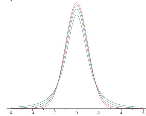
The \(t\) distribution is very similar to the normal distribution when the estimate of variance is based on many degrees of freedom, but has relatively more scores in its tails when there are fewer degrees of freedom. Figure \(\PageIndex{1}\) shows \(t\) distributions with \(2\), \(4\), and \(10\) degrees of freedom and the standard normal distribution. Notice that the normal distribution has relatively more scores in the center of the distribution and the \(t\) distribution has relatively more in the tails. The \(t\) distribution is therefore leptokurtic. The \(t\) distribution approaches the normal distribution as the degrees of freedom increase.

Figure \(\PageIndex{1}\): A comparison of \(t\) distributions with \(2\), \(4\), and \(10\) \(df\) and the standard normal distribution. The distribution with the lowest peak is the \(2\; df\) distribution, the next lowest is \(4\; df\), the lowest after that is \(10\; df\), and the highest is the standard normal distribution

Since the \(t\) distribution is leptokurtic, the percentage of the distribution within \(1.96\) standard deviations of the mean is less than the \(95\%\) for the normal distribution. Table \(\PageIndex{1}\) shows the number of standard deviations from the mean required to contain \(95\%\) and \(99\%\) of the area of the \(t\) distribution for various degrees of freedom. These are the values of \(t\) that you use in a confidence interval. The corresponding values for the normal distribution are \(1.96\) and \(2.58\) respectively. Notice that with few degrees of freedom, the values of \(t\) are much higher than the corresponding values for a normal distribution and that the difference decreases as the degrees of freedom increase. The values in Table \(\PageIndex{1}\) can be obtained from the "Find \(t\) for a confidence interval" calculator.

Table \(\PageIndex{1}\): Abbreviated \(t\) table

df	0.95	0.99
2	4.303	9.925
3	3.182	5.841
4	2.776	4.604
5	2.571	4.032
8	2.306	3.355
10	2.228	3.169
20	2.086	2.845
50	2.009	2.678
100	1.984	2.626

Returning to the problem posed at the beginning of this section, suppose you sampled \(9\) values from a normal population and estimated the standard error of the mean (\(\sigma _M\)) with \(s_M\). What is the probability that \(M\) would be within \(1.96 s_M\) of \(\mu\)? Since the sample size is \(9\), there are \(N - 1 = 8 df\). From Table \(\PageIndex{1}\) you can see that with \(8 df\) the probability is \(0.95\) that the mean will be within \(2.306 s_M\) of \(\mu\). The probability that it will be within \(1.96 s_M\) of \(\mu\) is therefore lower than \(0.95\).

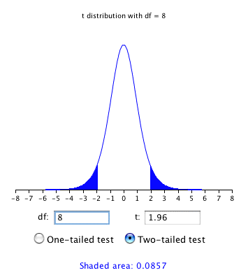
As shown in Figure \(\PageIndex{2}\), the "\(t\) distribution" calculator can be used to find that \(0.086\) of the area of a \(t\) distribution is more than \(1.96\) standard deviations from the mean, so the probability that \(M\) would be less than \(1.96 s_M\) from \(\mu\) is \(1 - 0.086 = 0.914\).

Figure \(\PageIndex{2}\): Area more than \(1.96\) standard deviations from the mean in a \(t\) distribution with \(8 df\). Note that the two-tailed button is selected so that the area in both tails will be included

As expected, this probability is less than \(0.95\) that would have been obtained if \(\sigma _M\) had been known instead of estimated.