
5.3: Skew and Kurtosis
- Page ID
- 3967

There are two more descriptive statistics that you will sometimes see reported in the psychological literature, known as skew and kurtosis. In practice, neither one is used anywhere near as frequently as the measures of central tendency and variability that we’ve been talking about. Skew is pretty important, so you do see it mentioned a fair bit; but I’ve actually never seen kurtosis reported in a scientific article to date.
## [1] -0.9174977## [1] 0.009023979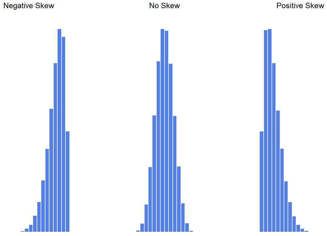
## [1] 0.9250898Since it’s the more interesting of the two, let’s start by talking about the skewness. Skewness is basically a measure of asymmetry, and the easiest way to explain it is by drawing some pictures. As Figure 5.4 illustrates, if the data tend to have a lot of extreme small values (i.e., the lower tail is “longer” than the upper tail) and not so many extremely large values (left panel), then we say that the data are negatively skewed. On the other hand, if there are more extremely large values than extremely small ones (right panel) we say that the data are positively skewed. That’s the qualitative idea behind skewness. The actual formula for the skewness of a data set is as follows
\[\text { skewness }(X)=\dfrac{1}{N \hat{\sigma}\ ^{3}} \sum_{i=1}^{N}\left(X_{i}-\bar{X}\right)^{3} \label{skew}\]
where N is the number of observations, \(\bar{X}\) is the sample mean, and \(\hat{\sigma}\) is the standard deviation (the “divide by N−1” version, that is). Perhaps more helpfully, it might be useful to point out that the psych package contains a skew() function that you can use to calculate skewness. So if we wanted to use this function to calculate the skewness of the afl.margins data, we’d first need to load the package
library( psych )which now makes it possible to use the following command:
skew( x = afl.margins ) ## [1] 0.7671555Not surprisingly, it turns out that the AFL winning margins data is fairly skewed.
The final measure that is sometimes referred to is the kurtosis of a data set. Put simply, kurtosis is a measure of the “tailedness”, or outlier character, of the data. Historically, it was thought that this statistic measures “pointiness” or “flatness” of a distribution, but this has been shown to be an error of interpretation. See Figure 5.5.
## [1] -0.9631805 ## [1] 0.02226287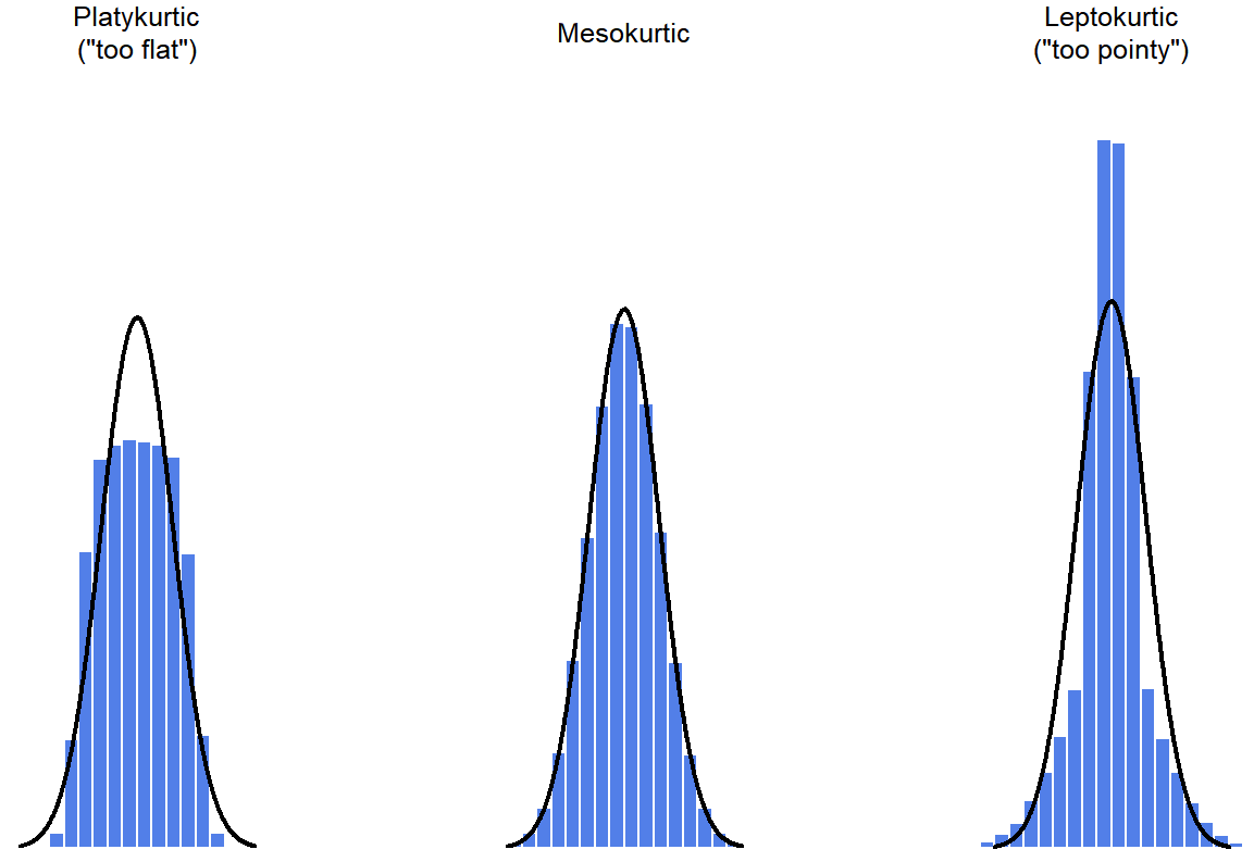
## [1] 1.994329 By mathematical calculations, the “normal curve” (black lines) has zero kurtosis, so the outlier character of a data set is assessed relative to this curve. In this Figure, the data on the left are less outlier-prone, so the kurtosis is negative and we call the data platykurtic. The data on the right are more outlier-prone, so the kurtosis is positive and we say that the data is leptokurtic. But the data in the middle are similar in their outlier character, so we say that it is mesokurtic and has kurtosis zero. This is summarised in the table below:
| informal term | technical name | kurtosis value |
|---|---|---|
| just pointy enough | mesokurtic | zero |
| too pointy | leptokurtic | positive |
| too flat | platykurtic | negative |
The equation for kurtosis is pretty similar in spirit to the formulas we’ve seen already for the variance and the skewness (Equation \ref{skew}); except that where the variance involved squared deviations and the skewness involved cubed deviations, the kurtosis involves raising the deviations to the fourth power:75
\[\text { kurtosis }(X)=\dfrac{1}{N \hat{\sigma}\ ^{4}} \sum_{i=1}^{N}\left(X_{i}-\bar{X}\right)^{4}-3\]
The psych package has a function called kurtosi() that you can use to calculate the kurtosis of your data. For instance, if we were to do this for the AFL margins,
kurtosi( x = afl.margins )## [1] 0.02962633we discover that the AFL winning margins data are just pointy enough.
Contributors
- Danielle Navarro (Associate Professor (Psychology) at University of New South Wales)
- Peter H. Westfall (Paul Whitfield Horn Professor and James and Marguerite Niver Professor, Texas Tech University)