2.7: Skew and Kurtosis
- Page ID
- 17304
\( \newcommand{\vecs}[1]{\overset { \scriptstyle \rightharpoonup} {\mathbf{#1}} } \)
\( \newcommand{\vecd}[1]{\overset{-\!-\!\rightharpoonup}{\vphantom{a}\smash {#1}}} \)
\( \newcommand{\id}{\mathrm{id}}\) \( \newcommand{\Span}{\mathrm{span}}\)
( \newcommand{\kernel}{\mathrm{null}\,}\) \( \newcommand{\range}{\mathrm{range}\,}\)
\( \newcommand{\RealPart}{\mathrm{Re}}\) \( \newcommand{\ImaginaryPart}{\mathrm{Im}}\)
\( \newcommand{\Argument}{\mathrm{Arg}}\) \( \newcommand{\norm}[1]{\| #1 \|}\)
\( \newcommand{\inner}[2]{\langle #1, #2 \rangle}\)
\( \newcommand{\Span}{\mathrm{span}}\)
\( \newcommand{\id}{\mathrm{id}}\)
\( \newcommand{\Span}{\mathrm{span}}\)
\( \newcommand{\kernel}{\mathrm{null}\,}\)
\( \newcommand{\range}{\mathrm{range}\,}\)
\( \newcommand{\RealPart}{\mathrm{Re}}\)
\( \newcommand{\ImaginaryPart}{\mathrm{Im}}\)
\( \newcommand{\Argument}{\mathrm{Arg}}\)
\( \newcommand{\norm}[1]{\| #1 \|}\)
\( \newcommand{\inner}[2]{\langle #1, #2 \rangle}\)
\( \newcommand{\Span}{\mathrm{span}}\) \( \newcommand{\AA}{\unicode[.8,0]{x212B}}\)
\( \newcommand{\vectorA}[1]{\vec{#1}} % arrow\)
\( \newcommand{\vectorAt}[1]{\vec{\text{#1}}} % arrow\)
\( \newcommand{\vectorB}[1]{\overset { \scriptstyle \rightharpoonup} {\mathbf{#1}} } \)
\( \newcommand{\vectorC}[1]{\textbf{#1}} \)
\( \newcommand{\vectorD}[1]{\overrightarrow{#1}} \)
\( \newcommand{\vectorDt}[1]{\overrightarrow{\text{#1}}} \)
\( \newcommand{\vectE}[1]{\overset{-\!-\!\rightharpoonup}{\vphantom{a}\smash{\mathbf {#1}}}} \)
\( \newcommand{\vecs}[1]{\overset { \scriptstyle \rightharpoonup} {\mathbf{#1}} } \)
\( \newcommand{\vecd}[1]{\overset{-\!-\!\rightharpoonup}{\vphantom{a}\smash {#1}}} \)
\(\newcommand{\avec}{\mathbf a}\) \(\newcommand{\bvec}{\mathbf b}\) \(\newcommand{\cvec}{\mathbf c}\) \(\newcommand{\dvec}{\mathbf d}\) \(\newcommand{\dtil}{\widetilde{\mathbf d}}\) \(\newcommand{\evec}{\mathbf e}\) \(\newcommand{\fvec}{\mathbf f}\) \(\newcommand{\nvec}{\mathbf n}\) \(\newcommand{\pvec}{\mathbf p}\) \(\newcommand{\qvec}{\mathbf q}\) \(\newcommand{\svec}{\mathbf s}\) \(\newcommand{\tvec}{\mathbf t}\) \(\newcommand{\uvec}{\mathbf u}\) \(\newcommand{\vvec}{\mathbf v}\) \(\newcommand{\wvec}{\mathbf w}\) \(\newcommand{\xvec}{\mathbf x}\) \(\newcommand{\yvec}{\mathbf y}\) \(\newcommand{\zvec}{\mathbf z}\) \(\newcommand{\rvec}{\mathbf r}\) \(\newcommand{\mvec}{\mathbf m}\) \(\newcommand{\zerovec}{\mathbf 0}\) \(\newcommand{\onevec}{\mathbf 1}\) \(\newcommand{\real}{\mathbb R}\) \(\newcommand{\twovec}[2]{\left[\begin{array}{r}#1 \\ #2 \end{array}\right]}\) \(\newcommand{\ctwovec}[2]{\left[\begin{array}{c}#1 \\ #2 \end{array}\right]}\) \(\newcommand{\threevec}[3]{\left[\begin{array}{r}#1 \\ #2 \\ #3 \end{array}\right]}\) \(\newcommand{\cthreevec}[3]{\left[\begin{array}{c}#1 \\ #2 \\ #3 \end{array}\right]}\) \(\newcommand{\fourvec}[4]{\left[\begin{array}{r}#1 \\ #2 \\ #3 \\ #4 \end{array}\right]}\) \(\newcommand{\cfourvec}[4]{\left[\begin{array}{c}#1 \\ #2 \\ #3 \\ #4 \end{array}\right]}\) \(\newcommand{\fivevec}[5]{\left[\begin{array}{r}#1 \\ #2 \\ #3 \\ #4 \\ #5 \\ \end{array}\right]}\) \(\newcommand{\cfivevec}[5]{\left[\begin{array}{c}#1 \\ #2 \\ #3 \\ #4 \\ #5 \\ \end{array}\right]}\) \(\newcommand{\mattwo}[4]{\left[\begin{array}{rr}#1 \amp #2 \\ #3 \amp #4 \\ \end{array}\right]}\) \(\newcommand{\laspan}[1]{\text{Span}\{#1\}}\) \(\newcommand{\bcal}{\cal B}\) \(\newcommand{\ccal}{\cal C}\) \(\newcommand{\scal}{\cal S}\) \(\newcommand{\wcal}{\cal W}\) \(\newcommand{\ecal}{\cal E}\) \(\newcommand{\coords}[2]{\left\{#1\right\}_{#2}}\) \(\newcommand{\gray}[1]{\color{gray}{#1}}\) \(\newcommand{\lgray}[1]{\color{lightgray}{#1}}\) \(\newcommand{\rank}{\operatorname{rank}}\) \(\newcommand{\row}{\text{Row}}\) \(\newcommand{\col}{\text{Col}}\) \(\renewcommand{\row}{\text{Row}}\) \(\newcommand{\nul}{\text{Nul}}\) \(\newcommand{\var}{\text{Var}}\) \(\newcommand{\corr}{\text{corr}}\) \(\newcommand{\len}[1]{\left|#1\right|}\) \(\newcommand{\bbar}{\overline{\bvec}}\) \(\newcommand{\bhat}{\widehat{\bvec}}\) \(\newcommand{\bperp}{\bvec^\perp}\) \(\newcommand{\xhat}{\widehat{\xvec}}\) \(\newcommand{\vhat}{\widehat{\vvec}}\) \(\newcommand{\uhat}{\widehat{\uvec}}\) \(\newcommand{\what}{\widehat{\wvec}}\) \(\newcommand{\Sighat}{\widehat{\Sigma}}\) \(\newcommand{\lt}{<}\) \(\newcommand{\gt}{>}\) \(\newcommand{\amp}{&}\) \(\definecolor{fillinmathshade}{gray}{0.9}\)Statisticians and researchers look at a lot of frequency charts (usually line graphs and histograms), so they know what to look for. Khan Academy has a great video previewing what will be discussed in this section.
Skew
Since it’s the more interesting of the two, let’s start by talking about the skew.
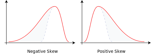
The shape of a frequency chart (line graph or histogram) can tell you a lot of about that data set. The simplest things to look for are any extreme scores (called outliers) that seem to be much higher or much lower than most of the other scores. These outliers may affect the shape of the distribution, making it skewed. A skewed distribution is one in which many scores are bunched up to one side, and there are only a few scores on the other side. A distribution can be positively skewed (meaning that the scores are bunched to the left, and the thin tail is pointing to the right) or negatively skewed (meaning that the scores are bunched to the right, and the thin tail is pointing to the left). Figure \(\PageIndex{1}\) shows examples of a positively skewed line graph (on the right) and a negatively skewed line graph on the left.
.png?revision=1)
Figure \(\PageIndex{1}\)- Diagram of Skew. (CC-BY-SA Rodolfo Hermans (Godot), CC BY-SA 3.0, via Wikimedia Commons)
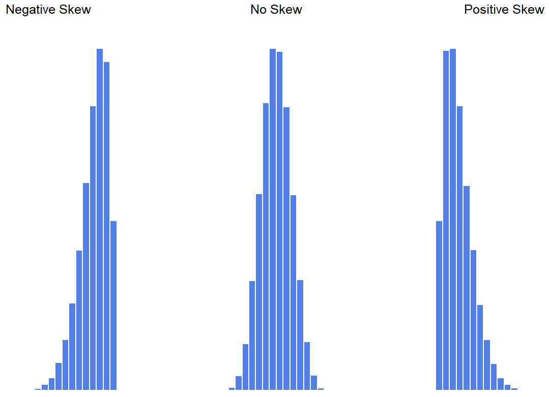
Skewness is basically a measure of asymmetry, and the easiest way to explain it is by drawing some pictures. As Figure \(\PageIndex{2}\) illustrates in histograms, if the data tend to have a lot of extreme small values (i.e., the lower tail is “longer” than the upper tail) and not so many extremely large values (left panel), then we say that the data are negatively skewed. On the other hand, if there are more extremely large values than extremely small ones (right panel) we say that the data are positively skewed. That’s the qualitative idea behind skewness.

Kurtosis
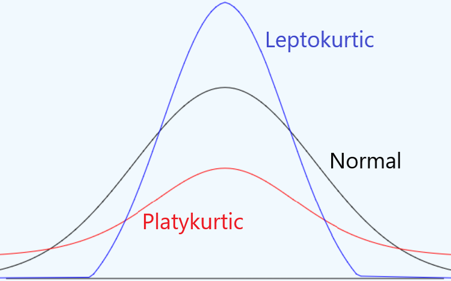
For distributions that are not skewed, you can look at how short and fat the distribution is, or if it is a medium bell-shaped curve, or if it is tall and narrow. This way of describing the shape of symmetrical (not-skewed) distributions, how broad the distribution is, is called kurtosis. Put simply, kurtosis is a measure of the “tailedness” of the data. As you can see in the line graph in Figure \(\PageIndex{3}\), there are three main types: wide, medium, or tall. Wide and flat graphs are called platykurtic. Medium, bell-shaped graphs are called mesokurtic or a normal distribution. Tall and narrow graphs are called leptokurtic.

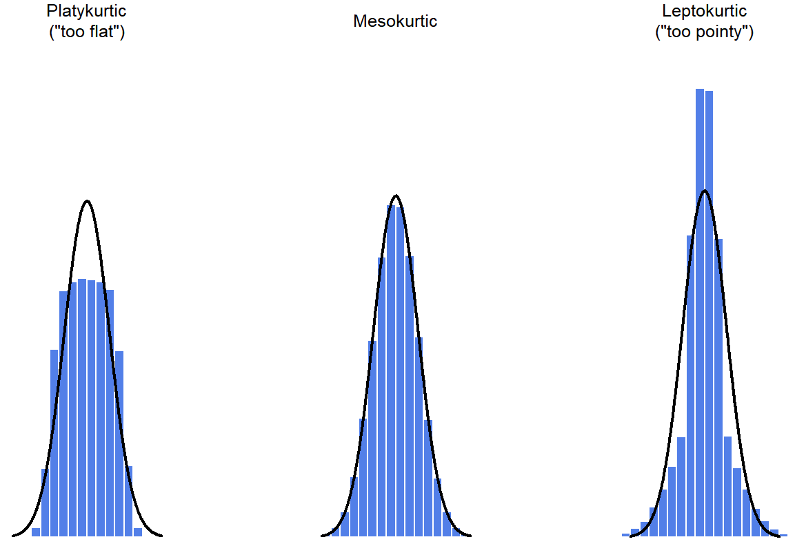
Figure \(\PageIndex{4}\) shows the three types of kurtosis in histograms. The histogram on the left shows platykurtic data, the middle histogram shows mesokurtic data, and on the right, we have a leptokurtic data set. By mathematical calculations, the “normal curve” (black lines) has zero kurtosis.

Figure \(\PageIndex{4}\): Diagram of Three Kurtosis Types in Histograms (CC-BY-SA Danielle Navarro from Learning Statistics with R)
The types of kurtosis are summarized in Table \(\PageIndex{1}\).
| Technical Name | Informal Description |
|---|---|
| mesokurtic | just pointy enough |
| leptokurtic | too pointy |
| platykurtic | too flat |
Summary
In practice, neither skew nor kurtosis is used anywhere near as frequently as the measures of central tendency and variability that will be discussed in next chapter. Skew is pretty important, though, so you do see it mentioned a fair bit; but I’ve actually never seen kurtosis reported in a scientific article to date
Contributors
- Danielle Navarro (University of New South Wales)
- Peter H. Westfall (Paul Whitfield Horn Professor and James and Marguerite Niver Professor, Texas Tech University)
- Figure \(\PageIndex{1}\) Image Attribution: Rodolfo Hermans (Godot), CC BY-SA 3.0, via Wikimedia Commons
- Figure \(\PageIndex{3}\) Image Attribution: CC-BY Larry Green from Lake Tahoe Community College


