3.1: Situation

In Chapter 2, tools for comparing the means of two groups were considered. More generally, these methods are used for a quantitative response and a categorical explanatory variable (group) which had two and only two levels. The complete overtake distance data set actually contained seven groups (Figure 3.1) with the outfit for each commute randomly assigned. In a situation with more than two groups, we have two choices. First, we could rely on our two group comparisons, performing tests for every possible pair (commute vs casual, casual vs highviz, commute vs highviz, …, polite vs racer), which would entail 21 different comparisons. But this would engage multiple testing issues and inflation of Type I error rates if not accounted for in some fashion. We would also end up with 21 p-values that answer detailed questions but none that addresses a simple but initially useful question – is there a difference somewhere among the pairs of groups or, under the null hypothesis, are all the true group means the same? In this chapter, we will learn a new method, called Analysis of Variance, ANOVA, or sometimes AOV that directly assesses evidence against the null hypothesis of no difference and then possibly leading to the ability to conclude that there is some overall difference in the means among the groups. This version of an ANOVA is called a One-Way ANOVA since there is just one⁵⁹ grouping variable. After we perform our One-Way ANOVA test for overall evidence of some difference, we will revisit the comparisons similar to those considered in Chapter 2 to get more details on specific differences among all the pairs of groups – what we call pair-wise comparisons. We will augment our previous methods for comparing two groups with an adjusted method for pairwise comparisons to make our results valid called Tukey’s Honest Significant Difference.

To make this more concrete, we return to the original overtake data, making a pirate-plot (Figure 3.1) as well as summarizing the overtake distances by the seven groups using favstats.

library(mosaic)
library(readr)
library(yarrr)
dd <- read_csv("http://www.math.montana.edu/courses/s217/documents/Walker2014_mod.csv")
dd <- dd %>% mutate(Condition = factor(Condition))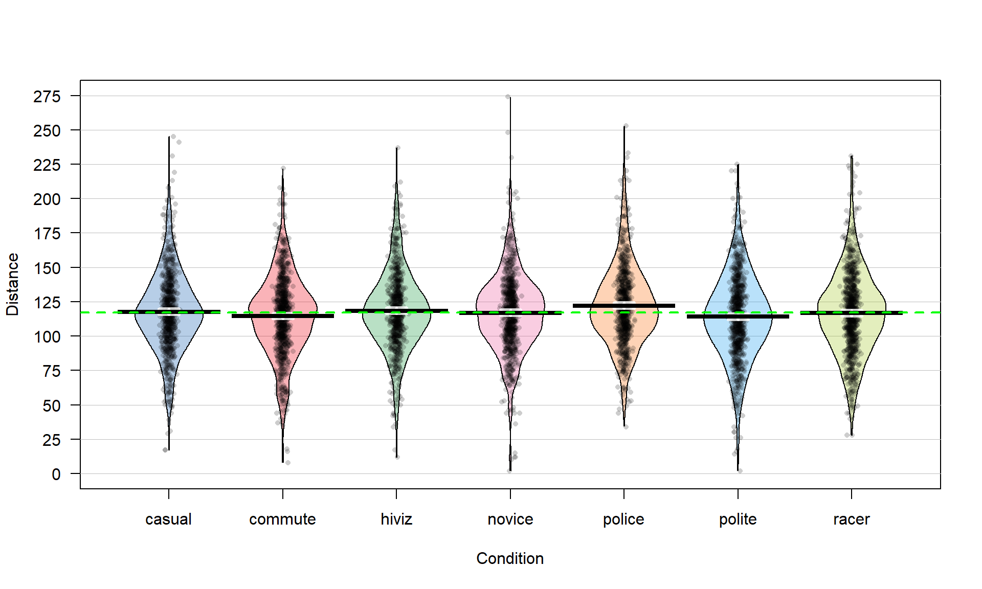

Figure 3.1: Pirate-plot of the overtake distances for the seven groups with group mean (bold lines with boxes indicating 95% confidence intervals) and the overall sample mean (dashed line) of 117.1 cm added.

pirateplot(Distance ~ Condition, data = dd, inf.method = "ci", inf.disp = "line")
abline(h = mean(dd$Distance), lwd = 2, col = "green", lty = 2) # Adds overall mean to plot

favstats(Distance ~ Condition, data = dd)

##   Condition min    Q1 median  Q3 max     mean       sd   n missing
## 1    casual  17 100.0    117 134 245 117.6110 29.86954 779       0
## 2   commute   8  98.0    116 132 222 114.6079 29.63166 857       0
## 3     hiviz  12 101.0    117 134 237 118.4383 29.03384 737       0
## 4    novice   2 100.5    118 133 274 116.9405 29.03812 807       0
## 5    police  34 104.0    119 138 253 122.1215 29.73662 790       0
## 6    polite   2  95.0    114 133 225 114.0518 31.23684 868       0
## 7     racer  28  98.0    117 135 231 116.7559 30.60059 852       0

There are slight differences in the sample sizes in the seven groups with between \(737\) and \(868\) observations, providing a data set has a total sample size of \(N = 5,690\). The sample means vary from 114.05 to 122.12 cm. In Chapter 2, we found moderate evidence regarding the difference in commute and casual. It is less clear whether we might find evidence of a difference between, say, commute and novice groups since we are comparing means of 114.05 and 116.94 cm. All the distributions appear to have similar shapes that are generally symmetric and bell-shaped and have relatively similar variability. The police vest group of observations seems to have highest sample mean, but there are many open questions about what differences might really exist here and there are many comparisons that could be considered.