3.6: Multiple (pair-wise) comparisons using Tukey’s HSD and the compact letter display

3.6 Multiple (pair-wise) comparisons using Tukey’s HSD and the compact letter display

With evidence against all the true means being equal and concluding that not all are equal, many researchers want to explore which groups show evidence of differing from one another. This provides information on the source of the overall difference that was detected and detailed information on which groups differed from one another. Because this is a shot-gun/unfocused sort of approach, some people think it is an over-used procedure. Others feel that it is an important method of addressing detailed questions about group comparisons in a valid and safe way. For example, we might want to know if OJ is different from VC at the 0.5 mg/day dosage level and these methods will allow us to get an answer to this sort of question. It also will test for differences between the OJ.0.5 and VC.2 groups and every other pair of levels that you can construct (15 total!). This method actually takes us back to the methods in Chapter 2 where we compared the means of two groups except that we need to deal with potentially many pair-wise comparisons, making an adjustment to account for that inflation in Type I errors that occurs due to many tests being performed at the same time. A commonly used method to make all the pair-wise comparisons that includes a correction for doing this is called Tukey’s Honest Significant Difference (Tukey’s HSD) method⁷⁴. The name suggests that not using it could lead to a dishonest answer and that it will give you an honest result. It is more that if you don’t do some sort of correction for all the tests you are performing, you might find some spurious⁷⁵ results. There are other methods that could be used to do a similar correction and also provide “honest” inferences; we are just going to learn one of them. Tukey’s method employs a different correction from the Bonferroni method discussed in Chapter 2 but also controls the family-wise error rate across all the pairs being compared.

In pair-wise comparisons between all the pairs of means in a One-Way ANOVA, the number of tests is based on the number of pairs. We can calculate the number of tests using \(J\) choose 2, \(\begin{pmatrix}J\\2\end{pmatrix}\), to get the number of unique pairs of size 2 that we can make out of \(J\) individual treatment levels. We don’t need to explore the combinatorics formula for this, as the choose function in R can give us the answers:

choose(3, 2)

## [1] 3

choose(4, 2)

## [1] 6

choose(5, 2)

## [1] 10

choose(6, 2)

## [1] 15

choose(7, 2)

## [1] 21

So if you have three groups (the smallest number where we have to worry about more than one pair), there are three unique pairs to compare. For six groups, like in the Guinea Pig study, we have to consider 15 tests to compare all the unique pairs of groups and with seven groups, there are 21 tests. Once there are more than two groups to compare, it seems like we should be worried about inflated family-wise error rates. Fortunately, the Tukey’s HSD method controls the family-wise error rate at your specified level (say 0.05) across any number of pair-wise comparisons. This means that the overall rate of at least one Type I error across all the tests is controlled at the specified significance level, often 5%. To do this, each test must use a slightly more conservative cut-off than if just one test is performed and the procedure helps us figure out how much more conservative we need to be.

Tukey’s HSD starts with focusing on the difference between the groups with the largest and smallest means (\(\bar{y}_{max}-\bar{y}_{min}\)). If \((\bar{y}_{max}-\bar{y}_{min}) \le \text{Margin of Error}\) for the difference in the means, then all other pairwise differences, say \(\vert \bar{y}_j - \bar{y}_{j'}\vert\), for two groups \(j\) and \(j'\), will be less than or equal to that margin of error. This also means that any confidence intervals for any difference in the means will contain 0. Tukey’s HSD selects a critical value so that (\(\bar{y}_{max}-\bar{y}_{min}\)) will be less than the margin of error in 95% of data sets drawn from populations with a common mean. This implies that in 95% of data sets in which all the population means are the same, all confidence intervals for differences in pairs of means will contain 0. Tukey’s HSD provides confidence intervals for the difference in true means between groups \(j\) and \(j'\), \(\mu_j-\mu_{j'}\), for all pairs where \(j \ne j'\), using

\[(\bar{y}_j - \bar{y}_{j'}) \mp \frac{q^*}{\sqrt{2}}\sqrt{\text{MS}_E\left(\frac{1}{n_j}+ \frac{1}{n_{j'}}\right)}\]

where \(\frac{q^*}{\sqrt{2}}\sqrt{\text{MS}_E\left(\frac{1}{n_j}+\frac{1}{n_{j'}}\right)}\) is the margin of error for the intervals. The distribution used to find the multiplier, \(q^*\), for the confidence intervals is available in the qtukey function and generally provides a slightly larger multiplier than the regular \(t^*\) from our two-sample \(t\)-based confidence interval discussed in Chapter 2. The formula otherwise is very similar to the one used in Chapter 2 with the SE for the difference in the means based on a measure of residual variance (here \(MS_E\)) times \(\left(\frac{1}{n_j}+\frac{1}{n_{j'}}\right)\) which weights the results based on the relative sample sizes in the groups.

We will use the confint, cld, and plot functions applied to output from the glht function (all from the multcomp package; Hothorn, Bretz, and Westfall (2008), (Hothorn, Bretz, and Westfall 2022)) to get the required comparisons from our ANOVA model. Unfortunately, its code format is a little complicated – but there are just two places to modify the code: include the model name and after mcp (stands for multiple comparison procedure) in the linfct option, you need to include the explanatory variable name as VARIABLENAME = "Tukey". The last part is to get the Tukey HSD multiple comparisons run on our explanatory variable⁷⁶. Once we obtain the intervals using the confint function or using plot applied to the stored results, we can use them to test \(H_0: \mu_j = \mu_{j'} \text{ vs } H_A: \mu_j \ne \mu_{j'}\) by assessing whether 0 is in the confidence interval for each pair. If 0 is in the interval, then there is weak evidence against the null hypothesis for that pair, so we do not detect a difference in that pair and do not conclude that there is a difference. If 0 is not in the interval, then we have strong evidence against \(H_0\) for that pair, detect a difference, and conclude that there is a difference in that pair at the specified family-wise significance level. You will see a switch to using the word “detection” to describe null hypotheses that we find strong evidence against as it can help to compactly write up these complicated results. The following code provides the numerical and graphical⁷⁷ results of applying Tukey’s HSD to the linear model for the Guinea Pig data:

library(multcomp)
Tm2 <- glht(m2, linfct = mcp(Treat = "Tukey"))

confint(Tm2)

## 
##   Simultaneous Confidence Intervals
## 
## Multiple Comparisons of Means: Tukey Contrasts
## 
## 
## Fit: lm(formula = len ~ Treat, data = ToothGrowth)
## 
## Quantile = 2.955
## 95% family-wise confidence level
##  
## 
## Linear Hypotheses:
##                      Estimate lwr      upr     
## VC.0.5 - OJ.0.5 == 0  -5.2500 -10.0490  -0.4510
## OJ.1 - OJ.0.5 == 0     9.4700   4.6710  14.2690
## VC.1 - OJ.0.5 == 0     3.5400  -1.2590   8.3390
## OJ.2 - OJ.0.5 == 0    12.8300   8.0310  17.6290
## VC.2 - OJ.0.5 == 0    12.9100   8.1110  17.7090
## OJ.1 - VC.0.5 == 0    14.7200   9.9210  19.5190
## VC.1 - VC.0.5 == 0     8.7900   3.9910  13.5890
## OJ.2 - VC.0.5 == 0    18.0800  13.2810  22.8790
## VC.2 - VC.0.5 == 0    18.1600  13.3610  22.9590
## VC.1 - OJ.1 == 0      -5.9300 -10.7290  -1.1310
## OJ.2 - OJ.1 == 0       3.3600  -1.4390   8.1590
## VC.2 - OJ.1 == 0       3.4400  -1.3590   8.2390
## OJ.2 - VC.1 == 0       9.2900   4.4910  14.0890
## VC.2 - VC.1 == 0       9.3700   4.5710  14.1690
## VC.2 - OJ.2 == 0       0.0800  -4.7190   4.8790

old.par <- par(mai = c(1,2,1,1)) #Makes room on the plot for the group names
plot(Tm2)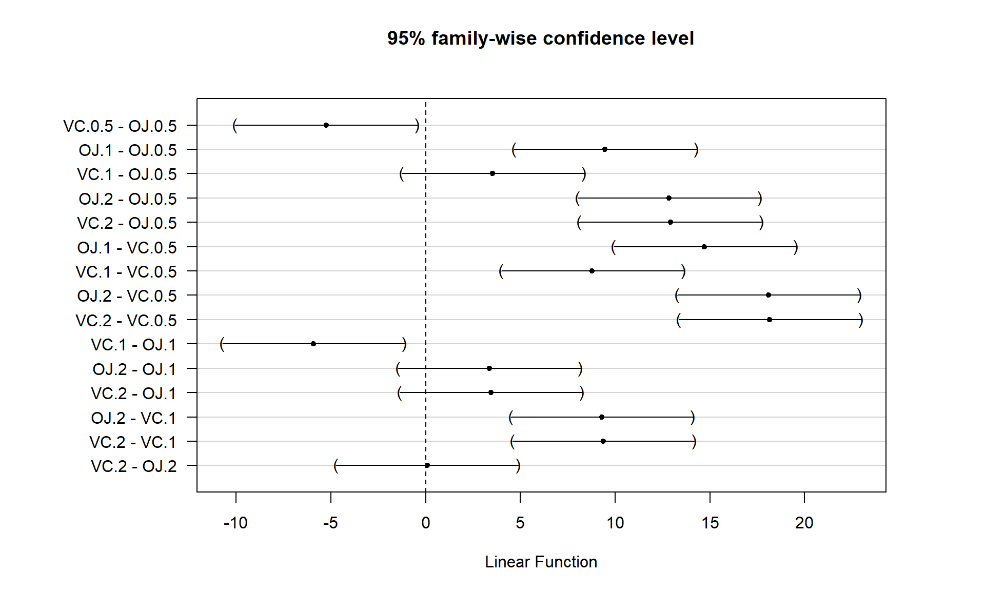

Figure 3.18: Graphical display of pair-wise comparisons from Tukey’s HSD for the Guinea Pig data. Any confidence intervals that do not contain 0 provide strong evidence against the null hypothesis of no difference in the true means for that pair of groups.

Figure 3.18 contains confidence intervals for the difference in the means for all 15 pairs of groups. For example, the first row in the plot contains the confidence interval for comparing VC.0.5 and OJ.0.5 (VC.0.5 minus OJ.0.5). In the numerical output, you can find that this 95% family-wise confidence interval goes from -10.05 to -0.45 microns (lwr and upr in the numerical output provide the CI endpoints). This interval does not contain 0 since its upper end point is -0.45 microns and so we can now say that there is strong evidence against the null hypothesis of no difference in this pair and that we detect that OJ and VC have different true mean growth rates at the 0.5 mg dosage level. We can go further and say that we are 95% confident that the difference in the true mean tooth growth between VC.0.5 and OJ.0.5 (VC.0.5-OJ.0.5) is between -10.05 and -0.45 microns, after adjusting for comparing all the pairs of groups. The center of this CI is -5.25 which is \(\widehat{\tau}_2\) and the estimate difference between VC.0.5 and the baseline category of OJ.0.5. That means we can get an un-adjusted 95% confidence interval from the confint function to compare to this adjusted CI. The interval that does not account for all the comparisons goes from -8.51 to -1.99 microns (second row out confint output), showing the increased width needed in Tukey’s interval to control the family-wise error rate when many pairs are being compared. With 14 other intervals, we obviously can’t give them all this much attention…

confint(m2)

##                  2.5 %    97.5 %
## (Intercept) 10.9276907 15.532309
## TreatVC.0.5 -8.5059571 -1.994043
## TreatOJ.1    6.2140429 12.725957
## TreatVC.1    0.2840429  6.795957
## TreatOJ.2    9.5740429 16.085957
## TreatVC.2    9.6540429 16.165957

If you put all these pair-wise tests together, you can generate an overall interpretation of Tukey’s HSD results that discusses sets of groups that are not detectably different from one another and those groups that were distinguished from other sets of groups. To do this, start with listing out the groups that are not detectably different (CIs contain 0), which, here, only occurs for four of the pairs. The CIs that contain 0 are for the pairs VC.1 and OJ.0.5, OJ.2 and OJ.1, VC.2 and OJ.1, and, finally, VC.2 and OJ.2. So VC.2, OJ.1, and OJ.2 are all not detectably different from each other and VC.1 and OJ.0.5 are also not detectably different. If you look carefully, VC.0.5 is detected as different from every other group. So there are basically three sets of groups that can be grouped together as “similar”: VC.2, OJ.1, and OJ.2; VC.1 and OJ.0.5; and VC.0.5. Sometimes groups overlap with some levels not being detectably different from other levels that belong to different groups and the story is not as clear as it is in this case. An example of this sort of overlap is seen in the next section.

There is a method that many researchers use to more efficiently generate and report these sorts of results that is called a compact letter display (CLD, Piepho (2004))⁷⁸. The cld function can be applied to the results from glht to generate the CLD that we can use to provide a “simple” summary of the sets of groups. In this discussion, we define a set as a union of different groups that can contain one or more members and the member of these groups are the different treatment levels.

cld(Tm2)

## OJ.0.5 VC.0.5   OJ.1   VC.1   OJ.2   VC.2 
##    "b"    "a"    "c"    "b"    "c"    "c"

Groups with the same letter are not detectably different (are in the same set) and groups that are detectably different get different letters (are in different sets). Groups can have more than one letter to reflect “overlap” between the sets of groups and sometimes a set of groups contains only a single treatment level (VC.0.5 is a set of size 1). Note that if the groups have the same letter, this does not mean they are the same, just that there is insufficient evidence to declare a difference for that pair. If we consider the previous output for the CLD, the “a” set contains VC.0.5, the “b” set contains OJ.0.5 and VC.1, and the “c” set contains OJ.1, OJ.2, and VC.2. These are exactly the groups of treatment levels that we obtained by going through all fifteen pairwise results.

One benefit of this work is that the CLD letters can be added to a plot (such as the pirate-plot) to help fully report the results and understand the sorts of differences Tukey’s HSD detected. The code with text involves placing text on the figure. In the text function, the x and y axis locations are specified (x-axis goes from 1 to 6 for the 6 categories) as well as the text to add (the CLD here). Some trial and error for locations may be needed to get the letters to be easily seen in a given pirate-plot. Figure 3.19 enhances the discussion by showing that the “a” group with VC.0.5 had the lowest average tooth growth, the “b” group had intermediate tooth growth for treatments OJ.0.5 and VC.1, and the highest growth rates came from OJ.1, OJ.2, and VC.2. Even though VC.2 had the highest average growth rate, we are not able to prove that its true mean is any higher than the other groups labeled with “c”. Hopefully the ease of getting to the story of the Tukey’s HSD results from a plot like this explains why it is common to report results using these methods instead of reporting 15 confidence intervals for all the pair-wise differences, either in a table or the plot.

# Options theme = 2,inf.f.o = 0,point.o = .5 added to focus on CLD
pirateplot(len ~ Treat, data = ToothGrowth, ylab = "Growth (microns)", inf.method = "ci",
           inf.disp = "line", theme = 2, inf.f.o = 0.3, point.o = .5) 
# CLD added to second bean (x = 2) at height of y = 10
text(x = 2, y = 10,"a", col = "blue", cex = 1.5)
# Adds "b" to first and fourth bean
text(x = c(1,4), y = c(15,18), "b", col = "red", cex = 1.5)
text(x = c(3,5,6), y = c(25,28,28), "c", col = "green", cex = 1.5) #Add "c" to three beans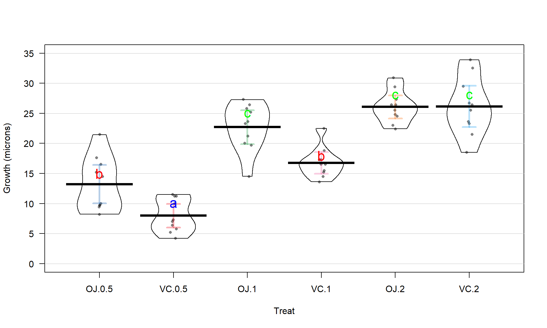

Figure 3.19: Pirate-plot of odontoblast growth by group with Tukey’s HSD compact letter display. Note some extra pirate-plot options are used to enhance focus on the CLD results.

There are just a couple of other details to mention on this set of methods. First, note that we interpret the set of confidence intervals simultaneously: We are 95% confident that ALL the intervals contain the respective differences in the true means (this is a family-wise interpretation). These intervals are adjusted from our regular two-sample \(t\) intervals that came from lm from Chapter 2 to allow this stronger interpretation. Specifically, they are wider. Second, if sample sizes are unequal in the groups, Tukey’s HSD is conservative and provides a family-wise error rate that is lower than the nominal (or specified) level. In other words, it fails less often than expected and the intervals provided are a little wider than needed, containing all the pairwise differences at higher than the nominal confidence level of (typically) 95%. Third, this is a parametric approach and violations of normality and constant variance will push the method in the other direction, potentially making the technique dangerously liberal. Nonparametric approaches to this problem are also possible, but will not be considered here.

Tukey’s HSD results can also be displayed as p-values for each pair-wise test result. This is a little less common but can allow you to directly assess the strength of evidence for a particular pair instead of using the detected/not result that the family-wise CIs provide. But the family-wise CIs are useful for exploring the size of the differences in the pairs and we need to simplify things to detect/not in these situations because there are so many tests. But if you want to see the Tukey HSD p-values, you can use

summary(Tm2)

## 
##   Simultaneous Tests for General Linear Hypotheses
## 
## Multiple Comparisons of Means: Tukey Contrasts
## 
## 
## Fit: lm(formula = len ~ Treat, data = ToothGrowth)
## 
## Linear Hypotheses:
##                      Estimate Std. Error t value Pr(>|t|)
## VC.0.5 - OJ.0.5 == 0   -5.250      1.624  -3.233  0.02424
## OJ.1 - OJ.0.5 == 0      9.470      1.624   5.831  < 0.001
## VC.1 - OJ.0.5 == 0      3.540      1.624   2.180  0.26411
## OJ.2 - OJ.0.5 == 0     12.830      1.624   7.900  < 0.001
## VC.2 - OJ.0.5 == 0     12.910      1.624   7.949  < 0.001
## OJ.1 - VC.0.5 == 0     14.720      1.624   9.064  < 0.001
## VC.1 - VC.0.5 == 0      8.790      1.624   5.413  < 0.001
## OJ.2 - VC.0.5 == 0     18.080      1.624  11.133  < 0.001
## VC.2 - VC.0.5 == 0     18.160      1.624  11.182  < 0.001
## VC.1 - OJ.1 == 0       -5.930      1.624  -3.651  0.00739
## OJ.2 - OJ.1 == 0        3.360      1.624   2.069  0.31868
## VC.2 - OJ.1 == 0        3.440      1.624   2.118  0.29372
## OJ.2 - VC.1 == 0        9.290      1.624   5.720  < 0.001
## VC.2 - VC.1 == 0        9.370      1.624   5.770  < 0.001
## VC.2 - OJ.2 == 0        0.080      1.624   0.049  1.00000
## (Adjusted p values reported -- single-step method)

These reinforce the strong evidence for many of the pairs and less strong evidence for four pairs that were not detected to be different. So these p-values provide another method to employ to report the Tukey’s HSD results – you would only need to report and explore the confidence intervals or the p-values, not both.

Tukey’s HSD does not require you to find a small p-value from your overall \(F\)-test to employ the methods but if you apply it to situations with p-values larger than your a priori significance level, you are unlikely to find any pairs that are detected as being different. Some statisticians suggest that you shouldn’t employ follow-up tests such as Tukey’s HSD when there is not much evidence against the overall null hypothesis. If you needed to use a permutation approach for your overall F-test, there are techniques for generating multiple-comparison adjusted permutation confidence intervals, but they are beyond the scope of this material. Using the tools here there are two options. First, you can subset the data set and do pairwise two-sample t-tests for all combinations of pairs of levels and apply a Bonferroni correction for the p-values that this would generate (this is more conservative than employing Tukey’s adjustments). Another alternative to be able to employ Tukey’s HSD as discussed here is to try to use a transformation on the response variable (things like logs or square-roots) so that the parametric approach is reasonable to use; transformations are discussed in Sections 7.5 and 7.6.