3.7: Pair-wise comparisons for the Overtake data

3.7 Pair-wise comparisons for the Overtake data

In our previous work with the overtake data, the overall ANOVA test led to a conclusion that there is some difference in the true means across the seven groups with a p-value < 0.001 giving very strong evidence against the null hypothesis of them all being equal. The original authors followed up their overall \(F\)-test with comparing every pair of outfits using one of the other methods for multiple testing adjustments available in the p.adjust function and detected differences between the police outfit and all others except for hiviz and no other pairs had p-values less than 0.05 using their approach. We will employ the Tukey’s HSD approach to address the same exploration and get basically the same results as they obtained, as well as estimated differences in the means in all the pairs of groups.

The code is similar⁷⁹ to the previous example focusing on the Condition variable for the 21 pairs to compare. To make these results easier to read and generally to make all the results with seven groups easier to understand, we can sort the levels of the explanatory based on the values in the response, using something like the means or medians of the responses for the groups. This does not change the analyses (the \(F\)-statistic and all pair-wise comparisons are the same), it just sorts them to be easier to discuss. Note that it might change the baseline group so would impact the reference-coded model even though the fitted values are the same. Specifically, we can use the reorder function based on the mean using something like reorder(FACTORVARIABLE, RESPONSEVARIABLE, FUN = mean), with our pipe and mutate functions used to modify the Condition variable. I like to put this “reordered” factor into a new variable so I can always go back to the other version if I want it but you could also re-write the original version with this modification – this only impacts the underlying order of the factor levels, not the entries for the observations themselves. The code here creates Condition2 and checks the levels for it and the original Condition variable, which shows the change in the order of the levels of the two factor variables:

dd <- dd %>% mutate(Condition2 = reorder(Condition, Distance, FUN = mean))

levels(dd$Condition)

## [1] "casual"  "commute" "hiviz"   "novice"  "police"  "polite"  "racer"

levels(dd$Condition2)

## [1] "polite"  "commute" "racer"   "novice"  "casual"  "hiviz"   "police"

And to verify that this worked, we can compare the means based on Condition and Condition2, and now it is even more clear which groups have the smallest and largest mean passing distances:

mean(Distance ~ Condition, data = dd)

##   casual  commute    hiviz   novice   police   polite    racer 
## 117.6110 114.6079 118.4383 116.9405 122.1215 114.0518 116.7559

mean(Distance ~ Condition2, data = dd)

##   polite  commute    racer   novice   casual    hiviz   police 
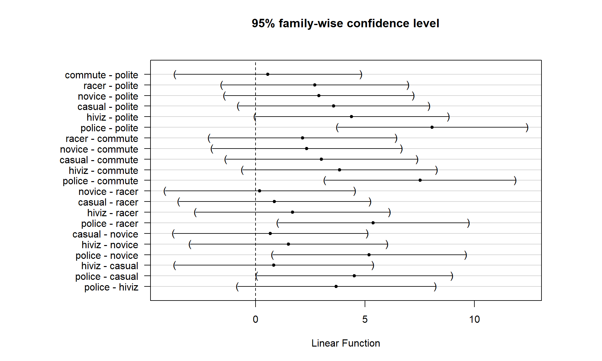
## 114.0518 114.6079 116.7559 116.9405 117.6110 118.4383 122.1215

In Figure 3.20, the 95% family-wise confidence intervals are displayed. There are only five pairs that have confidence intervals that do not contain 0 and all contain comparisons of the police group with others. So there is a detectable difference between police and polite, commute, racer, novice, and casual. The police versus casual comparison is hard to see whether 0 is in the interval or not in the plot, but the confidence interval goes from 0.06 to 8.97 cm (look at the results from confint), so suggests sufficient evidence to detect a difference in these groups (barely!) at the 5% family-wise significance level.

Figure 3.20: Tukey’s HSD confidence interval results at the 95% family-wise confidence level for the overtake distances linear model using the new Condition2 explanatory variable.

lm2 <- lm(Distance ~ Condition2, data = dd)
library(multcomp)
TmOV <- glht(lm2, linfct = mcp(Condition2 = "Tukey"))

confint(TmOv)

## 
##   Simultaneous Confidence Intervals
## 
## Multiple Comparisons of Means: Tukey Contrasts
## 
## 
## Fit: lm(formula = Distance ~ Condition2, data = dd)
## 
## Quantile = 2.9486
## 95% family-wise confidence level
##  
## 
## Linear Hypotheses:
##                       Estimate lwr      upr     
## commute - polite == 0  0.55609 -3.69182  4.80400
## racer - polite == 0    2.70403 -1.55015  6.95820
## novice - polite == 0   2.88868 -1.42494  7.20230
## casual - polite == 0   3.55920 -0.79441  7.91281
## hiviz - polite == 0    4.38642 -0.03208  8.80492
## police - polite == 0   8.06968  3.73207 12.40728
## racer - commute == 0   2.14793 -2.11975  6.41562
## novice - commute == 0  2.33259 -1.99435  6.65952
## casual - commute == 0  3.00311 -1.36370  7.36991
## hiviz - commute == 0   3.83033 -0.60118  8.26183
## police - commute == 0  7.51358  3.16273 11.86443
## novice - racer == 0    0.18465 -4.14844  4.51774
## casual - racer == 0    0.85517 -3.51773  5.22807
## hiviz - racer == 0     1.68239 -2.75512  6.11991
## police - racer == 0    5.36565  1.00868  9.72262
## casual - novice == 0   0.67052 -3.76023  5.10127
## hiviz - novice == 0    1.49774 -2.99679  5.99227
## police - novice == 0   5.18100  0.76597  9.59603
## hiviz - casual == 0    0.82722 -3.70570  5.36015
## police - casual == 0   4.51048  0.05637  8.96458
## police - hiviz == 0    3.68326 -0.83430  8.20081

cld(TmOv, abseps = 0.1)

##  polite commute   racer  novice  casual   hiviz  police 
##     "a"     "a"     "a"     "a"     "a"    "ab"     "b"

# Makes room on the plot for the group names, the second number of 2.5 is most 
# often adjusted: larger values provide more room on the left of the plot.
# Order is Bottom, Left, Top, Right (clockwise starting from the bottom).
old.par <- par(mai = c(1,2.5,1,1)) 
plot(TmOv)

The CLD also reinforces the previous discussion of which levels were detected as different and elucidates the other aspects of the results. Specifically, police is in a group with hiviz only (group “b”, not detectably different). But hiviz is also in a group with all the other levels so also is in group “a”. Figure 3.21 adds the CLD to the pirate-plot with the sorted means to help visually present these results with the original data, reiterating the benefits of sorting factor levels to make these plots easier to read. To wrap up this example (finally), we can see that we found that there was clear evidence against the null hypothesis of no difference in the true means, so concluded that there was some difference. The follow-up explorations show that we can really only suggest that the police outfit has detectably different mean distances and that is only for five of the six other levels. So if you are bike commuter (in the UK near London?), you are left to consider the size of this difference. The biggest estimated mean difference was 8.07 cm (3.2 inches) between police and polite. Do you think it is worth this potential extra average distance, especially given the wide variability in the distances, to make and then wear this vest? It is interesting that this result is found but it also is a fairly minimal size of a difference. It required an extremely large data set to detect these differences because the differences in the means are not very large relative to the variability in the responses. It seems like there might be many other reasons for why overtake distances vary that were not included our suite of predictors (they explored traffic volume in the paper as one other factor but we don’t have that in our data set) or maybe it is just unexplainably variable. But it makes me wonder whether it matters what I wear when I bike and whether it has an impact that matters for average overtake distances – even in the face of these “statistically significant” results. But maybe there is an impact on the “close calls” as you can see some differences in the lower tails of the distributions across the groups. The authors looked at the rates of “closer” overtakes by classifying the distances as either less than 100 cm (39.4 inches) as closer or not and also found some interesting results. Chapter 5 discusses a method called a Chi-square test of Homogeneity that would be appropriate here and allow for an analysis of the rates of closer passes and this study is revisited in the Practice Problems (Section 5.14) there. It ends up showing that rates of “closer passes” are smallest in the police group.

pirateplot(Distance ~ Condition2, data = dd, ylab = "Distance (cm)", inf.method = "ci",
           inf.disp = "line", theme = 2) 
text(x = 1:5,y = 200,"a",col = "blue",cex = 1.5) #CLD added
text(x = 5.9,y = 210,"a",col = "blue",cex = 1.5)
text(x = 6.1,y = 210,"b",col = "red",cex = 1.5)
text(x = 7,y = 215,"b",col = "red",cex = 1.5)

Figure 3.21: Pirate-plot of overtake distances by group, sorted by sample means with Tukey’s HSD CLD displayed.