3.3: One-Way ANOVA Sums of Squares, Mean Squares, and F-test

Last updated
Save as PDF

Page ID: 33230

\( \newcommand{\vecs}[1]{\overset { \scriptstyle \rightharpoonup} {\mathbf{#1}} } \) \( \newcommand{\vecd}[1]{\overset{-\!-\!\rightharpoonup}{\vphantom{a}\smash {#1}}} \)\(\newcommand{\id}{\mathrm{id}}\) \( \newcommand{\Span}{\mathrm{span}}\) \( \newcommand{\kernel}{\mathrm{null}\,}\) \( \newcommand{\range}{\mathrm{range}\,}\) \( \newcommand{\RealPart}{\mathrm{Re}}\) \( \newcommand{\ImaginaryPart}{\mathrm{Im}}\) \( \newcommand{\Argument}{\mathrm{Arg}}\) \( \newcommand{\norm}[1]{\| #1 \|}\) \( \newcommand{\inner}[2]{\langle #1, #2 \rangle}\) \( \newcommand{\Span}{\mathrm{span}}\) \(\newcommand{\id}{\mathrm{id}}\) \( \newcommand{\Span}{\mathrm{span}}\) \( \newcommand{\kernel}{\mathrm{null}\,}\) \( \newcommand{\range}{\mathrm{range}\,}\) \( \newcommand{\RealPart}{\mathrm{Re}}\) \( \newcommand{\ImaginaryPart}{\mathrm{Im}}\) \( \newcommand{\Argument}{\mathrm{Arg}}\) \( \newcommand{\norm}[1]{\| #1 \|}\) \( \newcommand{\inner}[2]{\langle #1, #2 \rangle}\) \( \newcommand{\Span}{\mathrm{span}}\)\(\newcommand{\AA}{\unicode[.8,0]{x212B}}\)

3.3 One-Way ANOVA Sums of Squares, Mean Squares, and F-test

The previous discussion showed two ways of parameterizing models for the One-Way ANOVA model and getting estimates from output but still hasn’t addressed how to assess evidence related to whether the observed differences in the means among the groups is “real”. In this section, we develop what is called the ANOVA F-test that provides a method of aggregating the differences among the means of 2 or more groups and testing (assessing evidence against) our null hypothesis of no difference in the means vs the alternative. In order to develop the test, some additional notation is needed. The sample size in each group is denoted \(n_j\) and the total sample size is \(\boldsymbol{N = \Sigma n_j = n_1 + n_2 + \ldots + n_J}\) where \(\Sigma\) (capital sigma) means “add up over whatever follows”. An estimated residual (\(e_{ij}\)) is the difference between an observation, \(y_{ij}\), and the model estimate, \(\widehat{y}_{ij} = \widehat{\mu}_j\), for that observation, \(y_{ij}-\widehat{y}_{ij} = e_{ij}\). It is basically what is left over that the mean part of the model (\(\widehat{\mu}_{j}\)) does not explain. It is also a window into how “good” the model might be because it reflects what the model was unable to explain.

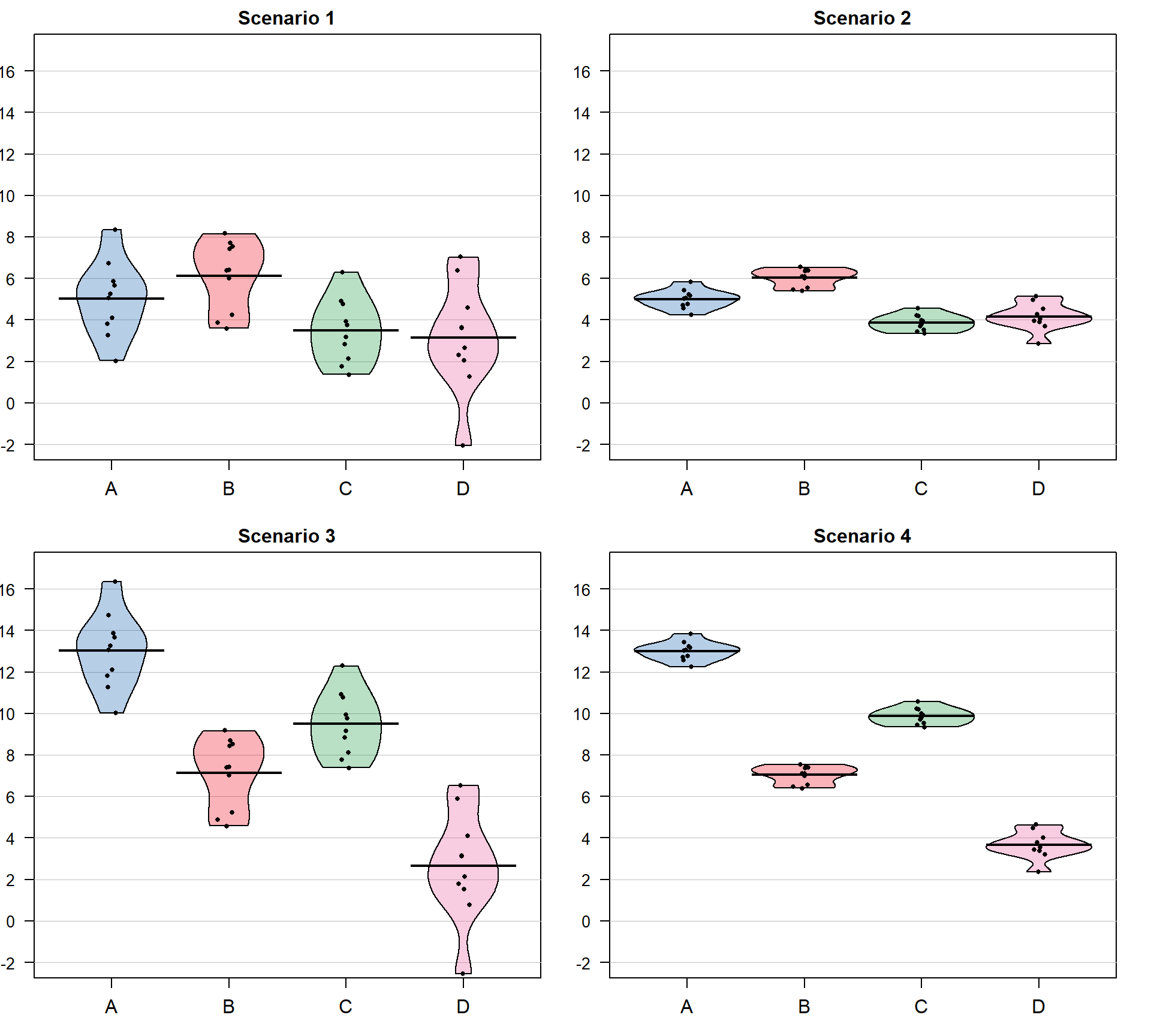
Consider the four different fake results for a situation with four groups (\(J = 4\)) displayed in Figure 3.3. Which of the different results shows the most and least evidence of differences in the means? In trying to answer this, think about both how different the means are (obviously important) and how variable the results are around the mean. These situations were created to have the same means in Scenarios 1 and 2 as well as matching means in Scenarios 3 and 4. In Scenarios 1 and 2, the differences in the means is smaller than in the other two results. But Scenario 2 should provide more evidence of what little difference is present than Scenario 1 because it has less variability around the means. The best situation for finding group differences here is Scenario 4 since it has the largest difference in the means and the least variability around those means. Our test statistic somehow needs to allow a comparison of the variability in the means to the overall variability to help us get results that reflect that Scenario 4 has the strongest evidence of a difference (most variability in the means and least variability around those means) and Scenario 1 would have the least evidence (least variability in the means and most variability around those means).

Figure 3.3: Demonstration of different amounts of difference in means relative to variability. Scenarios have the same means in rows and same variance around means in columns of plot. Confidence intervals not reported in the pirate-plots.

The statistic that allows the comparison of relative amounts of variation is called the ANOVA F-statistic. It is developed using sums of squares which are measures of total variation like those that are used in the numerator of the standard deviation (\(\Sigma_1^N(y_i-\bar{y})^2\)) that took all the observations, subtracted the mean, squared the differences, and then added up the results over all the observations to generate a measure of total variability. With multiple groups, we will focus on decomposing that total variability (Total Sums of Squares) into variability among the means (we’ll call this Explanatory Variable \(\mathbf{A}\textbf{'s}\) Sums of Squares) and variability in the residuals or errors (Error Sums of Squares). We define each of these quantities in the One-Way ANOVA situation as follows:

\(\textbf{SS}_{\textbf{Total}} =\) Total Sums of Squares \(= \Sigma^J_{j = 1}\Sigma^{n_j}_{i = 1}(y_{ij}-\bar{\bar{y}})^2\)
- This is the total variation in the responses around the grand mean (\(\bar{\bar{y}}\), the estimated mean for all the observations and available from the mean-only model).
- By summing over all \(n_j\) observations in each group, \(\Sigma^{n_j}_{i = 1}(\ )\), and then adding those results up across the groups, \(\Sigma^J_{j = 1}(\ )\), we accumulate the variation across all \(N\) observations.
- Note: this is the residual variation if the null model is used, so there is no further decomposition possible for that model.
- This is also equivalent to the numerator of the sample variance, \(\Sigma^{N}_{1}(y_{i}-\bar{y})^2\) which is what you get when you ignore the information on the potential differences in the groups.
\(\textbf{SS}_{\textbf{A}} =\) Explanatory Variable A’s Sums of Squares \(=\Sigma^J_{j = 1}\Sigma^{n_j}_{i = 1}(\bar{y}_{j}-\bar{\bar{y}})^2 = \Sigma^J_{j = 1}n_j(\bar{y}_{j}-\bar{\bar{y}})^2\)
- This is the variation in the group means around the grand mean based on the explanatory variable \(A\).
- This is also called sums of squares for the treatment, regression, or model.
\(\textbf{SS}_\textbf{E} =\) Error (Residual) Sums of Squares \(=\Sigma^J_{j = 1}\Sigma^{n_j}_{i = 1}(y_{ij}-\bar{y}_j)^2 = \Sigma^J_{j = 1}\Sigma^{n_j}_{i = 1}(e_{ij})^2\)
- This is the variation in the responses around the group means.
- Also called the sums of squares for the residuals, especially when using the second version of the formula, which shows that it is just the squared residuals added up across all the observations.

The possibly surprising result given the mass of notation just presented is that the total sums of squares is ALWAYS equal to the sum of explanatory variable \(A\text{'s}\) sum of squares and the error sums of squares,

\[\textbf{SS}_{\textbf{Total}} \mathbf{=} \textbf{SS}_\textbf{A} \mathbf{+} \textbf{SS}_\textbf{E}.\]

This result is called the sums of squares decomposition formula. The equality implies that if the \(\textbf{SS}_\textbf{A}\) goes up, then the \(\textbf{SS}_\textbf{E}\) must go down if \(\textbf{SS}_{\textbf{Total}}\) remains the same. We use these results to build our test statistic and organize this information in what is called an ANOVA table. The ANOVA table is generated using the anova function applied to the reference-coded model, lm2:

lm2 <- lm(Distance ~ Condition, data = dd)
anova(lm2)

## Analysis of Variance Table
## 
## Response: Distance
##             Df  Sum Sq Mean Sq F value    Pr(>F)
## Condition    6   34948  5824.7  6.5081 7.392e-07
## Residuals 5683 5086298   895.0

Note that the ANOVA table has a row labeled Condition, which contains information for the grouping variable (we’ll generally refer to this as explanatory variable \(A\) but here it is the outfit group that was randomly assigned), and a row labeled Residuals, which is synonymous with “Error”. The Sums of Squares (SS) are available in the Sum Sq column. It doesn’t show a row for “Total” but the \(\textbf{SS}_{\textbf{Total}} \mathbf{=} \textbf{SS}_\textbf{A} \mathbf{+} \textbf{SS}_\textbf{E} = 5,121,246\).

34948 + 5086298

## [1] 5121246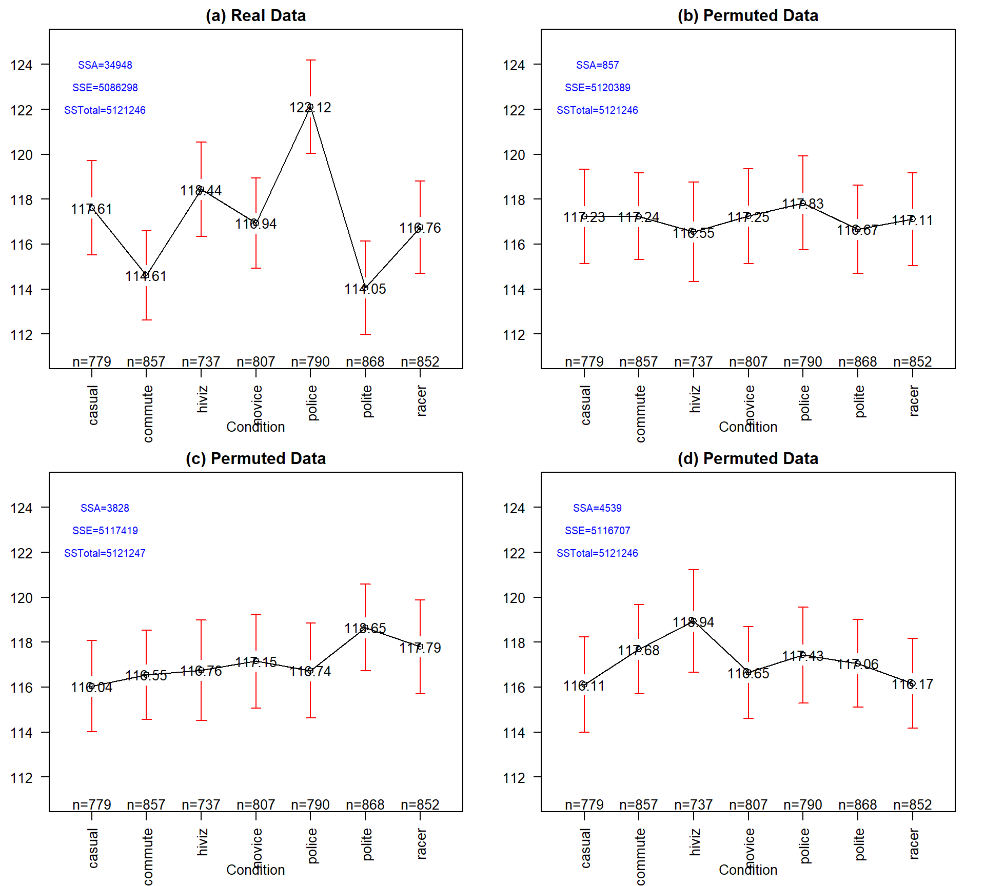

Plot of means and 95% confidence intervals for the three groups for the real overtake data (a) and three different permutations of the outfit group labels to the same responses in (b), (c), and (d). Note that SSTotal is always the same but the different amounts of variation associated with the means (SSA) or the errors (SSE) changes in permutation. — Figure 3.4: Plot of means and 95% confidence intervals for the three groups for the real overtake data (a) and three different permutations of the outfit group labels to the same responses in (b), (c), and (d). Note that `SSTotal` is always the same but the different amounts of variation associated with the means (`SSA`) or the errors (`SSE`) changes in permutation.

It may be easiest to understand the sums of squares decomposition by connecting it to our permutation ideas. In a permutation situation, the total variation (\(SS_\text{Total}\)) cannot change – it is the same responses varying around the same grand mean. However, the amount of variation attributed to variation among the means and in the residuals can change if we change which observations go with which group. In Figure 3.4 (panel a), the means, sums of squares, and 95% confidence intervals for each mean are displayed for the seven groups from the original overtake data. Three permuted versions of the data set are summarized in panels (b), (c), and (d). The \(\text{SS}_A\) is 34948 in the real data set and between 857 and 4539 in the permuted data sets. If you had to pick among the plots for the one with the most evidence of a difference in the means, you hopefully would pick panel (a). This visual “unusualness” suggests that this observed result is unusual relative to the possibilities under permutations, which are, again, the possibilities tied to having the null hypothesis being true. But note that the differences here are not that great between these three permuted data sets and the real one. It is likely that at least some might have selected panel (d) as also looking like it shows some evidence of differences, although the variation in the means in the real data set is clearly more pronounced than in this or the other permutations.

One way to think about \(\textbf{SS}_\textbf{A}\) is that it is a function that converts the variation in the group means into a single value. This makes it a reasonable test statistic in a permutation testing context. By comparing the observed \(\text{SS}_A =\) 34948 to the permutation results of 857, 3828, and 4539 we see that the observed result is much more extreme than the three alternate versions. In contrast to our previous test statistics where positive and negative differences were possible, \(\text{SS}_A\) is always positive with a value of 0 corresponding to no variation in the means. The larger the \(\text{SS}_A\), the more variation there is in the means. The permutation p-value for the alternative hypothesis of some (not of greater or less than!) difference in the true means of the groups will involve counting the number of permuted \(SS_A^*\) results that are as large or larger than what we observed.

To do a permutation test, we need to be able to calculate and extract the \(\text{SS}_A\) value. In the ANOVA table, it is the second number in the first row; we can use the bracket, [,], referencing to extract that number from the ANOVA table that anova produces with anova(lm(Distance ~ Condition, data = dd))[1, 2]. We’ll store the observed value of \(\text{SS}_A\) in Tobs, reusing some ideas from Chapter 2.

Tobs <- anova(lm(Distance ~ Condition, data = dd))[1,2]; Tobs

## [1] 34948.43

The following code performs the permutations B = 1,000 times using the shuffle function, builds up a vector of results in Tobs, and then makes a plot of the resulting permutation distribution:

Figure 3.5: Histogram and density curve of permutation distribution of \(\text{SS}_A\) with the observed value of \(\text{SS}_A\) displayed as a bold, vertical line. The proportion of results that are as large or larger than the observed value of \(\text{SS}_A\) provides an estimate of the p-value.

B <- 1000
Tstar <- matrix(NA, nrow = B)
for (b in (1:B)){
  Tstar[b] <- anova(lm(Distance ~ shuffle(Condition), data = dd))[1,2]
  }
tibble(Tstar) %>%  ggplot(aes(x = Tstar)) + 
  geom_histogram(aes(y = ..ncount..), bins = 20, col = 1, fill = "skyblue") + 
  geom_density(aes(y = ..scaled..)) +
  theme_bw() +
  labs(y = "Density") +
  geom_vline(xintercept = Tobs, col = "red", lwd = 2) +
  stat_bin(aes(y = ..ncount.., label = ..count..), bins = 20, 
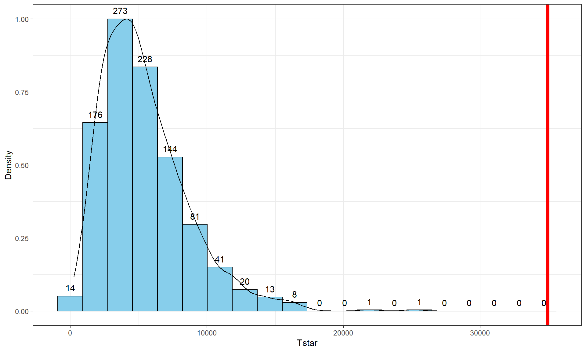
           geom = "text", vjust = -0.75)

The right-skewed distribution (Figure 3.5) contains the distribution of \(\text{SS}^*_A\text{'s}\) under permutations (where all the groups are assumed to be equivalent under the null hypothesis). The observed result is larger than all of the \(\text{SS}^*_A\text{'s}\). The proportion of permuted results that exceed the observed value is found using pdata as before, except only for the area to the right of the observed result. We know that Tobs will always be positive so no absolute values are required here.

pdata(Tstar, Tobs, lower.tail = F)[[1]]

## [1] 0

Because there were no permutations that exceeded the observed value, the p-value should be reported as p-value < 0.001 (less than 1 in 1,000) and not 0. This suggests very strong evidence against the null hypothesis of no difference in the true means. We would interpret this p-value as saying that there is less than a 0.1% chance of getting a \(\text{SS}_A\) as large or larger than we observed, given that the null hypothesis is true.

It ends up that some nice parametric statistical results are available (if our assumptions are met) for the ratio of estimated variances, the estimated variances are called Mean Squares. To turn sums of squares into mean square (variance) estimates, we divide the sums of squares by the amount of free information available. For example, remember the typical variance estimator introductory statistics, \(\Sigma^N_1(y_i-\bar{y})^2/(N-1)\)? Your instructor probably spent some time trying various approaches to explaining why the denominator is the sample size minus 1. The most useful explanation for our purposes moving forward is that we “lose” one piece of information to estimate the mean and there are \(N\) deviations around the single mean so we divide by \(N-1\). The main point is that the sums of squares were divided by something and we got an estimator for the variance, in that situation for the observations overall.

Now consider \(\text{SS}_E = \Sigma^J_{j = 1}\Sigma^{n_j}_{i = 1}(y_{ij}-\bar{y}_j)^2\) which still has \(N\) deviations but it varies around the \(J\) means, so the

\[\textbf{Mean Square Error} = \text{MS}_E = \text{SS}_E/(N-J).\]

Basically, we lose \(J\) pieces of information in this calculation because we have to estimate \(J\) means. The similar calculation of the Mean Square for variable \(\mathbf{A}\) (\(\text{MS}_A\)) is harder to see in the formula (\(\text{SS}_A = \Sigma^J_{j = 1}n_j(\bar{y}_i-\bar{\bar{y}})^2\)), but the same reasoning can be used to understand the denominator for forming \(\text{MS}_A\): there are \(J\) means that vary around the grand mean so

\[\text{MS}_A = \text{SS}_A/(J-1).\]

In summary, the two mean squares are simply:

\(\text{MS}_A = \text{SS}_A/(J-1)\), which estimates the variance of the group means around the grand mean.
\(\text{MS}_{\text{Error}} = \text{SS}_{\text{Error}}/(N-J)\), which estimates the variation of the errors around the group means.

These results are put together using a ratio to define the ANOVA F-statistic (also called the F-ratio) as:

\[F = \text{MS}_A/\text{MS}_{\text{Error}}.\]

If the variability in the means is “similar” to the variability in the residuals, the statistic would have a value around 1. If that variability is similar then there would be no evidence of a difference in the means. If the \(\text{MS}_A\) is much larger than the \(\text{MS}_E\), the \(F\)-statistic will provide evidence against the null hypothesis. The “size” of the \(F\)-statistic is formalized by finding the p-value. The \(F\)-statistic, if assumptions discussed below are not violated and we assume the null hypothesis is true, follows what is called an \(F\)-distribution. The F-distribution is a right-skewed distribution whose shape is defined by what are called the numerator degrees of freedom (\(J-1\)) and the denominator degrees of freedom (\(N-J\)). These names correspond to the values that we used to calculate the mean squares and where in the \(F\)-ratio each mean square was used; \(F\)-distributions are denoted by their degrees of freedom using the convention of \(F\) (numerator df, denominator df). Some examples of different \(F\)-distributions are displayed for you in Figure 3.6.

The characteristics of the F-distribution can be summarized as:

Right skewed,
Nonzero probabilities for values greater than 0,
Its shape changes depending on the numerator DF and denominator DF, and
Always use the right-tailed area for p-values.

Figure 3.6: Density curves of four different \(F\)-distributions. Upper left is an \(F(6, 5683)\), upper right is \(F(2, 10)\), lower left is \(F(6, 10)\), and lower right is \(F(3, 20)\). P-values are found using the areas to the right of the observed \(F\)-statistic value in all F-distributions.

Now we are ready to discuss an ANOVA table since we know about each of its components. Note the general format of the ANOVA table is in Table 3.2⁶⁴:

Table 3.2: General One-Way ANOVA table.
Source	DF	Sums of Squares	Mean Squares	F-ratio	P-value
Variable A	\(J-1\)	\(\text{SS}_A\)	\(\text{MS}_A = \text{SS}_A/(J-1)\)	\(F = \text{MS}_A/\text{MS}_E\)	Right tail of \(F(J-1,N-J)\)
Residuals	\(N-J\)	\(\text{SS}_E\)	\(\text{MS}_E = \text{SS}_E/(N-J)\)
Total	\(N-1\)	\(\text{SS}_{\text{Total}}\)

The table is oriented to help you reconstruct the \(F\)-ratio from each of its components. The output from R is similar although it does not provide the last row and sometimes switches the order of columns in different functions we will use. The R version of the table for the type of outfit effect (Condition) with \(J = 7\) levels and \(N = 5,690\) observations, repeated from above, is:

anova(lm2)

## Analysis of Variance Table
## 
## Response: Distance
##             Df  Sum Sq Mean Sq F value       Pr(>F)
## Condition    6   34948  5824.7  6.5081 0.0000007392
## Residuals 5683 5086298   895.0

The p-value from the \(F\)-distribution is 0.0000007 so we can report it⁶⁵ as a p-value < 0.0001. We can verify this result using the observed \(F\)-statistic of 6.51 (which came from taking the ratio of the two mean squares, F = 5824.74/895) which follows an \(F(6, 5683)\) distribution if the null hypothesis is true and some other assumptions are met. Using the pf function provides us with areas in the specified \(F\)-distribution with the df1 provided to the function as the numerator df and df2 as the denominator df and lower.tail = F reflecting our desire for a right tailed area.

pf(6.51, df1 = 6, df2 = 5683, lower.tail = F)

## [1] 0.0000007353832

The result from the \(F\)-distribution using this parametric procedure is similar to the p-value obtained using permutations with the test statistic of the \(\text{SS}_A\), which was < 0.0001. The \(F\)-statistic obviously is another potential test statistic to use as a test statistic in a permutation approach, now that we know about it. We should check that we get similar results from it with permutations as we did from using \(\text{SS}_A\) as a permutation-test test statistic. The following code generates the permutation distribution for the \(F\)-statistic (Figure 3.7) and assesses how unusual the observed \(F\)-statistic of 6.51 was in this permutation distribution. The only change in the code involves moving from extracting \(\text{SS}_A\) to extracting the \(F\)-ratio which is in the 4^th column of the anova output:

Tobs <- anova(lm(Distance ~ Condition, data = dd))[1,4]; Tobs

## [1] 6.508071

B <- 1000
Tstar <- matrix(NA, nrow = B)
for (b in (1:B)){
  Tstar[b] <- anova(lm(Distance ~ shuffle(Condition), data = dd))[1,4]
}

pdata(Tstar, Tobs, lower.tail = F)[[1]]

## [1] 0

tibble(Tstar) %>%  ggplot(aes(x = Tstar)) + 
  geom_histogram(aes(y = ..ncount..), bins = 20, col = 1, fill = "skyblue") + 
  geom_density(aes(y = ..scaled..)) +
  theme_bw() +
  labs(y = "Density") +
  geom_vline(xintercept = Tobs, col = "red", lwd = 2) +
  stat_bin(aes(y = ..ncount.., label = ..count..), bins = 20, 
           geom = "text", vjust = -0.75)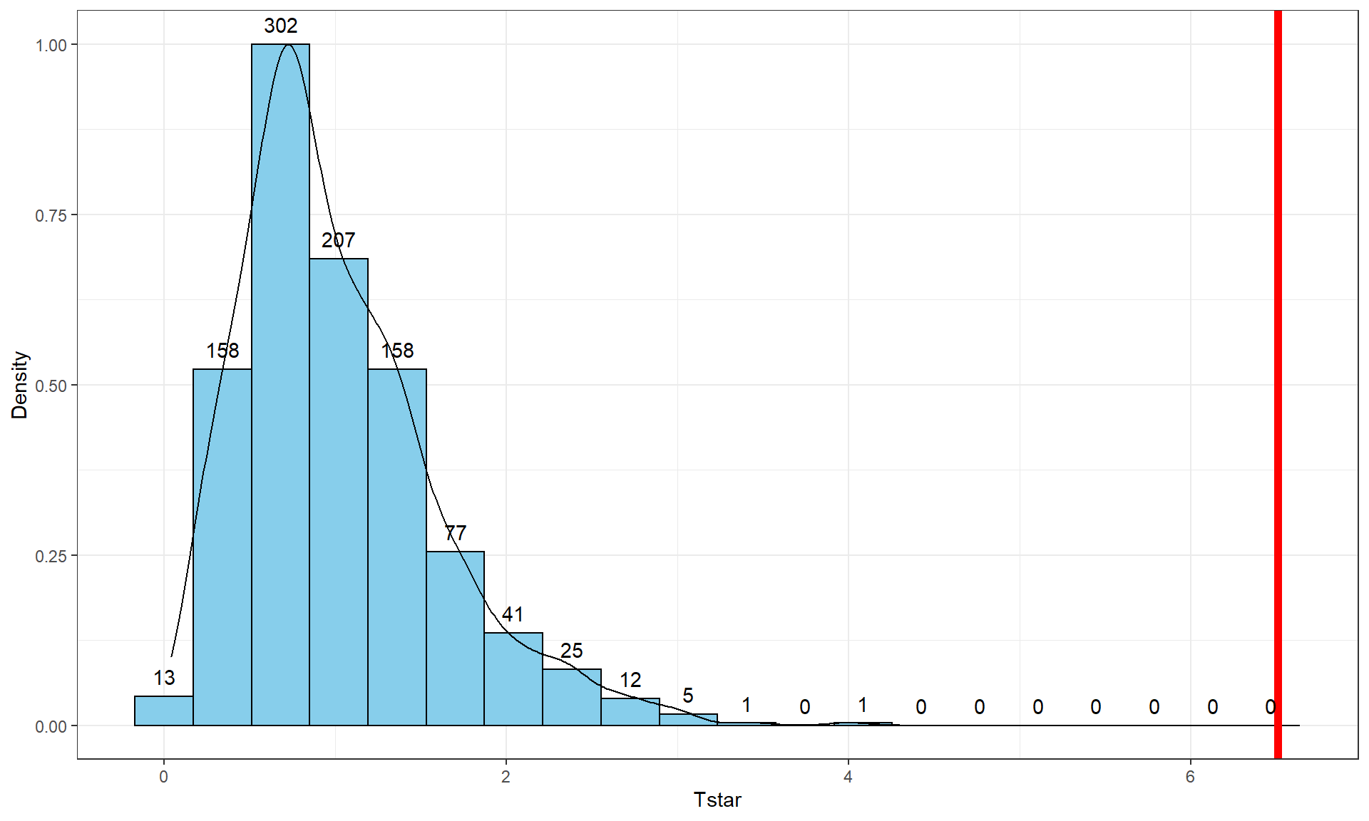

Figure 3.7: Histogram and density curve of the permutation distribution of the F-statistic with bold, vertical line for the observed value of the test statistic of 6.51.

The permutation-based p-value is again at less than 1 in 1,000, which matches the other results closely. The first conclusion is that using a test statistic of either the \(F\)-statistic or the \(\text{SS}_A\) provide similar permutation results. However, we tend to favor using the \(F\)-statistic because it is more commonly used in reporting ANOVA results, not because it is any better in a permutation context .

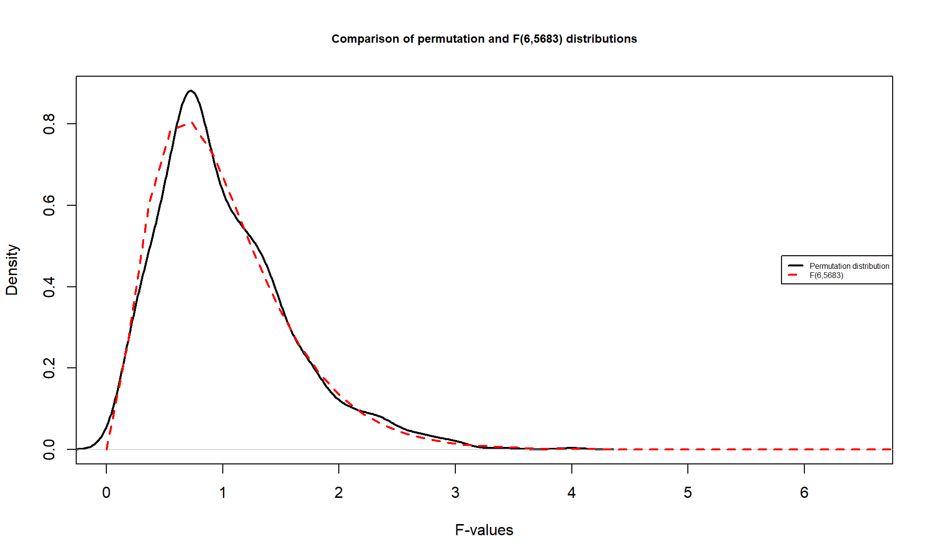
It is also interesting to compare the permutation distribution for the \(F\)-statistic and the parametric \(F(6, 6583)\) distribution (Figure 3.8). They do not match perfectly but are quite similar. Some the differences around 0 are due to the behavior of the method used to create the density curve and are not really a problem for the methods. The similarity in the two curves explains why both methods would give similar p-value results for almost any test statistic value. In some situations, the correspondence will not be quite so close.

Figure 3.8: Comparison of \(F(6, 6583)\) (dashed line) and permutation distribution (solid line).

So how can we rectify this result (p-value < 0.0001) and the Chapter 2 result that reported moderate evidence against the null hypothesis of no difference between commute and casual with a \(\text{p-value}\approx 0.04\)? I selected the two groups to compare in Chapter 2 because they were somewhat far apart but not too far apart. I could have selected police and polite as they are furthest apart and just focused on that difference. “Cherry-picking” a comparison when many are present, especially one that is most different, without accounting for this choice creates a false sense of the real situation and inflates the Type I error rate because of the selection⁶⁶. If the entire suite of pairwise comparisons are considered, this result may lose some of its luster. In other words, if we consider the suite of 21 pair-wise differences (and the tests) implicit in comparing all of them, we may need really strong evidence against the null in at least some of the pairs to suggest overall differences. In this situation, the hiviz and casual groups are not that different from each other so their difference does not contribute much to the overall \(F\)-test. In Section 3.6, we will revisit this topic and consider a method that is statistically valid for performing all possible pair-wise comparisons that is also consistent with our overall test results.