2.9: Confidence intervals and bootstrapping

Up to this point the focus has been on hypotheses, p-values, and estimates of the size of differences. But so far this has not explored inference techniques for the size of the difference. Confidence intervals provide an interval where we are __% confident that the true parameter lies. The idea of “confidence” is that if we repeated randomly sampling from the same population and made a similar confidence interval, the collection of all these confidence intervals would contain the true parameter at the specified confidence level (usually 95%). We only get to make one interval and so it either has the true parameter in it or not, and we don’t know the truth in real situations.

Confidence intervals can be constructed with parametric and a nonparametric approaches. The nonparametric approach will be using what is called bootstrapping and draws its name from “pull yourself up by your bootstraps” where you improve your situation based on your own efforts. In statistics, we make our situation or inferences better by re-using the observations we have by assuming that the sample represents the population. Since each observation represents other similar observations in the population that we didn’t get to measure, if we sample with replacement to generate a new data set of size n from our data set (also of size n) it mimics the process of taking repeated random samples of size \(n\) from our population of interest. This process also ends up giving us useful sampling distributions of statistics even when our standard normality assumption is violated, similar to what we encountered in the permutation tests. Bootstrapping is especially useful in situations where we are interested in statistics other than the mean (say we want a confidence interval for a median or a standard deviation) or when we consider functions of more than one parameter and don’t want to derive the distribution of the statistic (say the difference in two medians). Here, bootstrapping is used to provide more trustworthy inferences when some of our assumptions (especially normality) might be violated for our parametric confidence interval procedure.

To perform bootstrapping, the resample function from the mosaic package will be used. We can apply this function to a data set and get a new version of the data set by sampling new observations with replacement from the original one⁵². The new, bootstrapped version of the data set (called dsample_BTS below) contains a new variable called orig.id which is the number of the subject from the original data set. By summarizing how often each of these id’s occurred in a bootstrapped data set, we can see how the re-sampling works. The table function will count up how many times each observation was used in the bootstrap sample, providing a row with the id followed by a row with the count⁵³. In the first bootstrap sample shown, the 1^st, 14^th, and 26^th observations were sampled twice, the 9^th and 28^th observations were sampled four times, and the 4^th, 5^th, 6^th, and many others were not sampled at all. Bootstrap sampling thus picks some observations multiple times and to do that it has to ignore some⁵⁴ observations.

set.seed(406)
dsample_BTS <- resample(dsample)

table(as.numeric(dsample_BTS$orig.id))

## 
##  1  2  3  7  8  9 10 11 12 13 14 16 18 19 23 24 25 26 27 28 30 
##  2  1  1  1  1  4  1  1  1  1  2  1  1  1  1  1  1  2  1  4  1

Like in permutations, one randomization isn’t enough. A second bootstrap sample is also provided to help you get a sense of what bootstrap data sets contain. It did not select observations two through five but did select eight others more than once. You can see other variations in the resulting re-sampling of subjects with the most sampled observation used four times. With \(n = 30\), the chance of selecting any observation for any slot in the new data set is \(1/30\) and the expected or mean number of appearances we expect to see for an observation is the number of random draws times the probably of selection on each so \(30*1/30 = 1\). So we expect to see each observation in the bootstrap sample on average once but random variability in the samples then creates the possibility of seeing it more than once or not all.

dsample_BTS2 <- resample(dsample)
table(as.numeric(dsample_BTS2$orig.id))

## 
##  1  6  7  8  9 10 11 12 13 16 17 20 22 23 24 25 26 28 30 
##  2  2  1  1  2  1  4  1  3  1  1  1  2  2  1  1  2  1  1

We can use the two results to get an idea of distribution of results in terms of number of times observations might be re-sampled when sampling with replacement and the variation in those results, as shown in Figure 2.22. We could also derive the expected counts for each number of times of re-sampling when we start with all observations having an equal chance and sampling with replacement but this isn’t important for using bootstrapping methods.

Figure 2.22: Counts of number of times of observation (or not observed for times re-sampled of 0) for two bootstrap samples.

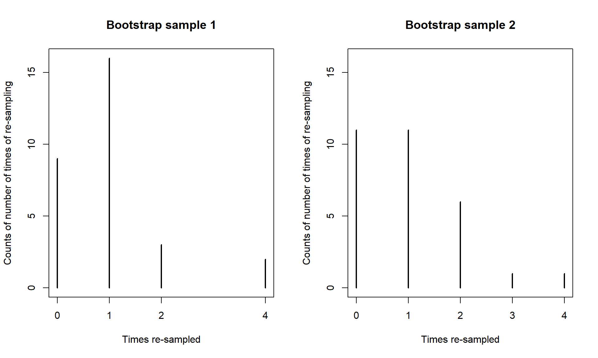
The main point of this exploration was to see that each run of the resample function provides a new version of the data set. Repeating this \(B\) times using another for loop, we will track our quantity of interest, say \(T\), in all these new “data sets” and call those results \(T^*\). The distribution of the bootstrapped \(T^*\) statistics tells us about the range of results to expect for the statistic. The middle % of the \(T^*\)’s provides a % bootstrap confidence interval⁵⁵ for the true parameter – here the difference in the two population means.

To make this concrete, we can revisit our previous examples, starting with the dsample data created before and our interest in comparing the mean passing distances for the commuter and casual outfit groups in the \(n = 30\) stratified random sample that was extracted. The bootstrapping code is very similar to the permutation code except that we apply the resample function to the entire data set used in lm as opposed to the shuffle function that was applied only to the explanatory variable.

lm1 <- lm(Distance ~ Condition, data = dsample)
Tobs <- coef(lm1)[2]; Tobs

## Conditioncommute 
##        -25.93333

B <- 1000
set.seed(1234)
Tstar <- matrix(NA, nrow = B)
for (b in (1:B)){
  lmP <- lm(Distance ~ Condition, data = resample(dsample))
  Tstar[b] <- coef(lmP)[2]
}

favstats(Tstar)

##        min        Q1    median        Q3      max      mean       sd    n missing
##  -66.96429 -34.57159 -25.65881 -17.12391 17.17857 -25.73641 12.30987 1000       0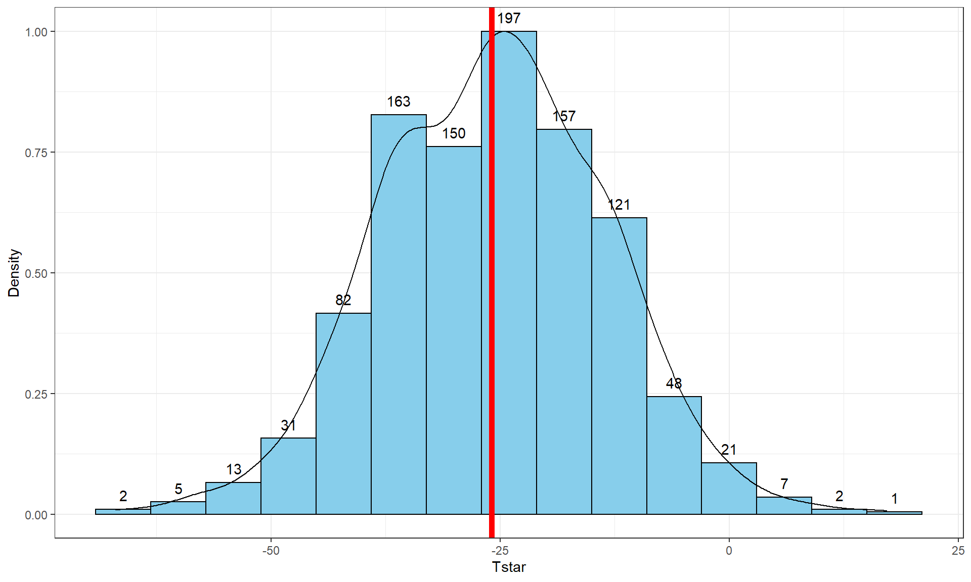

Figure 2.23: Histogram and density curve of bootstrap distributions of difference in sample mean Distances with vertical line for the observed difference in the means of -25.933.

tibble(Tstar) %>% ggplot(aes(x = Tstar)) + 
  geom_histogram(aes(y = ..ncount..), bins = 15, col = 1, fill = "skyblue", center = 0) + 
  geom_density(aes(y = ..scaled..)) +
  theme_bw() +
  labs(y = "Density") +
  geom_vline(xintercept = Tobs, col = "red", lwd = 2) +
  stat_bin(aes(y = ..ncount.., label = ..count..), bins = 15, 
           geom = "text", vjust = -0.75)

In this situation, the observed difference in the mean passing distances is -25.933 cm (commute - casual), which is the bold vertical line in Figure 2.23. The bootstrap distribution shows the results for the difference in the sample means when fake data sets are re-constructed by sampling from the original data set with replacement. The bootstrap distribution is approximately centered at the observed value (difference in the sample means) and is relatively symmetric.

The permutation distribution in the same situation (Figure 2.10) had a similar shape but was centered at 0. Permutations create sampling distributions based on assuming the null hypothesis is true, which is useful for hypothesis testing. Bootstrapping creates distributions centered at the observed result, which is the sampling distribution “under the alternative” or when no null hypothesis is assumed; bootstrap distributions are useful for generating confidence intervals for the true parameter values.

To create a 95% bootstrap confidence interval for the difference in the true mean distances (\(\mu_\text{commute}-\mu_\text{casual}\)), select the middle 95% of results from the bootstrap distribution. Specifically, find the 2.5^th percentile and the 97.5^th percentile (values that put 2.5 and 97.5% of the results to the left) in the bootstrap distribution, which leaves 95% in the middle for the confidence interval. To find percentiles in a distribution in R, functions are of the form q[Name of distribution], with the function qt extracting percentiles from a \(t\)-distribution (examples below). From the bootstrap results, use the qdata function on the Tstar results that contain the bootstrap distribution of the statistic of interest.

qdata(Tstar, 0.025)

##     2.5% 
## -50.0055

qdata(Tstar, 0.975)

##     97.5% 
## -2.248774

These results tell us that the 2.5^th percentile of the bootstrap distribution is at -50.006 cm and the 97.5^th percentile is at -2.249 cm. We can combine these results to provide a 95% confidence for \(\mu_\text{commute}-\mu_\text{casaual}\) that is between -50.01 and -2.25 cm. This interval is interpreted as with any confidence interval, that we are 95% confident that the difference in the true mean distances (commute minus casual groups) is between -50.01 and -2.25 cm. Or we can switch the direction of the comparison and say that we are 95% confident that the difference in the true means is between 2.25 and 50.01 cm (casual minus commute). This result would be incorporated into step 5 of the hypothesis testing protocol to accompany discussing the size of the estimated difference in the groups or used as a result of interest in itself. Both percentiles can be obtained in one line of code using:

quantiles <- qdata(Tstar, c(0.025,0.975))

quantiles

##       2.5%      97.5% 
## -50.005502  -2.248774

Figure 2.24 displays those same percentiles on the bootstrap distribution residing in Tstar.

Figure 2.24: Histogram and density curve of bootstrap distribution with 95% bootstrap confidence intervals displayed (bold, dashed vertical lines).

tibble(Tstar) %>% ggplot(aes(x = Tstar)) + 
  geom_histogram(aes(y = ..ncount..), bins = 15, col = 1, fill = "skyblue", center = 0) + 
  geom_density(aes(y = ..scaled..)) +
  theme_bw() +
  labs(y = "Density") +
  geom_vline(xintercept = quantiles, col = "blue", lwd = 2, lty = 2) +
  stat_bin(aes(y = ..ncount.., label = ..count..), bins = 15, 
           geom = "text", vjust = -0.75)

Although confidence intervals can exist without referencing hypotheses, we can revisit our previous hypotheses and see what this confidence interval tells us about the test of \(H_0: \mu_\text{commute} = \mu_\text{casual}\). This null hypothesis is equivalent to testing \(H_0: \mu_\text{commute} - \mu_\text{casual} = 0\), that the difference in the true means is equal to 0 cm. And the difference in the means was the scale for our confidence interval, which did not contain 0 cm. The 0 cm values is an interesting reference value for the confidence interval, because here it is the value where the true means are equal to each other (have a difference of 0 cm). In general, if our confidence interval does not contain 0, then it is saying that 0 is not one of the likely values for the difference in the true means at the selected confidence level. This implies that we should reject a claim that they are equal. This provides the same inferences for the hypotheses that we considered previously using both parametric and permutation approaches using a fixed \(\alpha\) approach where \(\alpha\) = 1 - confidence level.

The general summary is that we can use confidence intervals to test hypotheses by assessing whether the reference value under the null hypothesis is in the confidence interval (suggests insufficient evidence against \(H_0\) to reject it, at least at the \(\alpha\) level and equivalent to having a p-value larger than \(\alpha\)) or outside the confidence interval (sufficient evidence against \(H_0\) to reject it and equivalent to having a p-value that is less than \(\alpha\)). P-values are more informative about hypotheses (measure of evidence against the null hypothesis) but confidence intervals are more informative about the size of differences, so both offer useful information and, as shown here, can provide consistent conclusions about hypotheses. But it is best practice to use p-values to assess evidence against null hypotheses and confidence intervals to do inferences for the size of differences.

As in the previous situation, we also want to consider the parametric approach for comparison purposes and to have that method available, especially to help us understand some methods where we will only consider parametric inferences in later chapters. The parametric confidence interval is called the equal variance, two-sample t confidence interval and additionally assumes that the populations being sampled from are normally distributed instead of just that they have similar shapes in the bootstrap approach. The parametric method leads to using a \(t\)-distribution to form the interval with the degrees of freedom for the \(t\)-distribution of \(n-2\) although we can obtain it without direct reference to this distribution using the confint function applied to the lm model. This function generates two confidence intervals and the one in the second row is the one we are interested as it pertains to the difference in the true means of the two groups. The parametric 95% confidence interval here is from -51.6 to -0.26 cm which is a bit different in width from the nonparametric bootstrap interval that was from -50.01 and -2.25 cm.

confint(lm1)

##                      2.5 %      97.5 %
## (Intercept)      117.64498 153.9550243
## Conditioncommute -51.60841  -0.2582517

The bootstrap interval was narrower by almost 4 cm and its upper limit was much further from 0. The bootstrap CI can vary depending on the random number seed used and additional runs of the code produced intervals of (-49.6, -2.8), (-48.3, -2.5), and (-50.9, -1.1) so the differences between the parametric and nonparametric approaches was not just due to an unusual bootstrap distribution. It is not entirely clear why the two intervals differ but there are slightly more results in the left tail of Figure 2.24 than in the right tail and this shifts the 95% confidence slightly away from 0 as compared to the parametric approach. All intervals have the same interpretation, only the methods for calculating the intervals and the assumptions differ. Specifically, the bootstrap interval can tolerate different distribution shapes other than normal and still provide intervals that work well⁵⁶. The other assumptions are all the same as for the hypothesis test, where we continue to assume that we have independent observations with equal variances for the two groups and maintain concerns about inferences here due to the violation of independence in these responses.

The formula that lm is using to calculate the parametric equal variance, two-sample \(t\)-based confidence interval is:

\[\bar{x}_1 - \bar{x}_2 \mp t^*_{df}s_p\sqrt{\frac{1}{n_1}+\frac{1}{n_2}}\]

In this situation, the df is again \(n_1+n_2-2\) (the total sample size - 2) and \(s_p = \sqrt{\frac{(n_1-1)s_1^2 + (n_2-1)s_2^2}{n_1+n_2-2}}\). The \(t^*_{df}\) is a multiplier that comes from finding the percentile from the \(t\)-distribution that puts \(C\)% in the middle of the distribution with \(C\) being the confidence level. It is important to note that this \(t^*\) has nothing to do with the previous test statistic \(t\). It is confusing and students first engaging these two options often happily take the result from a test statistic calculation and use it for a multiplier in a \(t\)-based confidence interval – try to focus on which \(t\) you are interested in before you use either. Figure 2.25 shows the \(t\)-distribution with 28 degrees of freedom and the cut-offs that put 95% of the area in the middle.

Figure 2.25: Plot of \(t(28)\) with cut-offs for putting 95% of distribution in the middle that delineate the \(t^*\) multiplier to make a 95% confidence interval.

For 95% confidence intervals, the multiplier is going to be close to 2 and anything else is a likely indication of a mistake. We can use R to get the multipliers for confidence intervals using the qt function in a similar fashion to how qdata was used in the bootstrap results, except that this new value must be used in the previous confidence interval formula. This function produces values for requested percentiles, so if we want to put 95% in the middle, we place 2.5% in each tail of the distribution and need to request the 97.5^th percentile. Because the \(t\)-distribution is always symmetric around 0, we merely need to look up the value for the 97.5^th percentile and know that the multiplier for the 2.5^th percentile is just \(-t^*\). The \(t^*\) multiplier to form the confidence interval is 2.0484 for a 95% confidence interval when the \(df = 28\) based on the results from qt:

qt(0.975, df = 28)

## [1] 2.048407

Note that the 2.5^th percentile is just the negative of this value due to symmetry and the real source of the minus in the minus/plus in the formula for the confidence interval.

qt(0.025, df = 28)

## [1] -2.048407

We can also re-write the confidence interval formula into a slightly more general forms as

\[\bar{x}_1 - \bar{x}_2 \mp t^*_{df}SE_{\bar{x}_1 - \bar{x}_2}\ \text{ OR }\ \bar{x}_1 - \bar{x}_2 \mp ME\]

where \(SE_{\bar{x}_1 - \bar{x}_2} = s_p\sqrt{\frac{1}{n_1}+\frac{1}{n_2}}\) and \(ME = t^*_{df}SE_{\bar{x}_1 - \bar{x}_2}\). The SE is available in the lm model summary for the line related to the difference in groups in the “Std. Error” column. In some situations, researchers will report the standard error (SE) or margin of error (ME) as a method of quantifying the uncertainty in a statistic. The SE is an estimate of the standard deviation of the statistic (here \(\bar{x}_1 - \bar{x}_2\)) and the ME is an estimate of the precision of a statistic that can be used to directly form a confidence interval. The ME depends on the choice of confidence level although 95% is almost always selected.

To finish this example, R can be used to help you do calculations much like a calculator except with much more power “under the hood”. You have to make sure you are careful with using ( ) to group items and remember that the asterisk (*) is used for multiplication. We need the pertinent information which is available from the favstats output repeated below to calculate the confidence interval “by hand”⁵⁷ using R.

favstats(Distance ~ Condition, data = dsample)

##   Condition min    Q1 median    Q3 max     mean       sd  n missing
## 1    casual  72 112.5    143 154.5 208 135.8000 39.36133 15       0
## 2   commute  60  88.5    113 123.0 168 109.8667 28.41244 15       0

Start with typing the following command to calculate \(s_p\) and store it in a variable named sp:

sp <- sqrt(((15 - 1)*(39.36133^2) + (15 - 1)*(28.4124^2))/(15 + 15 - 2))
sp

## [1] 34.32622

Then calculate the confidence interval that confint provided using:

109.8667 - 135.8 + c(-1,1)*qt(0.975, df = 28)*sp*sqrt(1/15 + 1/15)

## [1] -51.6083698  -0.2582302

Or using the information from the model summary:

-25.933 + c(-1,1)*qt(0.975, df = 28)*12.534

## [1] -51.6077351  -0.2582649

The previous results all use c(-1, 1) times the margin of error to subtract and add the ME to the difference in the sample means (\(109.8667 - 135.8\)), which generates the lower and then upper bounds of the confidence interval. If desired, we can also use just the last portion of the calculation to find the margin of error, which is 25.675 here.

qt(0.975, df = 28)*sp*sqrt(1/15 + 1/15)

## [1] 25.67507

For the entire \(n = 1,636\) data set for these two groups, the results are obtained using the following code. The estimated difference in the means is -3 cm (commute minus casual). The \(t\)-based 95% confidence interval is from -5.89 to -0.11.

lm_all <- lm(Distance ~ Condition, data = ddsub)
confint(lm_all) #Parametric 95% CI

##                       2.5 %      97.5 %
## (Intercept)      115.520697 119.7013823
## Conditioncommute  -5.891248  -0.1149621

## Conditioncommute 
##        -3.003105

##        2.5%       97.5% 
## -5.81626474 -0.07606663

The bootstrap 95% confidence interval is from -5.816 to -0.076. With this large data set, the differences between parametric and permutation approaches decrease and they essentially equivalent here. The bootstrap distribution (not displayed) for the differences in the sample means is relatively symmetric and centered around the estimated difference of 6 cm. So using all the observations we would be 95% confident that the true mean difference in overtake distances (commute - casual) is between -5.82 and -0.08 cm, providing additional information about the estimated difference in the sample means of 6 cm.

Tobs <- coef(lm_all)[2]; Tobs

B <- 1000
set.seed(1234)
Tstar <- matrix(NA, nrow = B)
for (b in (1:B)){
  lmP <- lm(Distance ~ Condition, data = resample(ddsub))
  Tstar[b] <- coef(lmP)[2]
}

qdata(Tstar, c(0.025, 0.975))

##        2.5%       97.5% 
## -5.81626474 -0.07606663