2.8: Reproducibility Crisis - Moving beyond p < 0.05, publication bias, and multiple testing issues

In the previous examples, some variation in p-values was observed as different methods (parametric, nonparametric) were applied to the same data set and in the permutation approach, the p-values can vary as well from one set of permutations to another. P-values also vary based on randomness in the data that were collected – take a different (random) sample and you will get different data and a different p-value. We want the best estimate of a p-value we can obtain, so should use the best sampling method and inference technique that we can. But it is just an estimate of the evidence against the null hypothesis. These sources of variability make fixed \(\alpha\) NHST especially worry-some as sampling variability could take a p-value from just below to just above \(\alpha\) and this would lead to completely different inferences if the only focus is on rejecting the null hypothesis at a fixed significance level. But viewing p-values on a gradient from extremely strong (close to 0) to no (1) evidence against the null hypothesis, p-values of, say, 0.046 and 0.054 provide basically the same evidence against the null hypothesis. The fixed \(\alpha\) decision-making is tied into the use of the terminology of “significant results” or, slightly better, “statistically significant results” that are intended to convey that there was sufficient evidence to reject the null hypothesis at some pre-decided \(\alpha\) level. You will notice that this is the only time that the “s-word” (significant) is considered here.

The focus on p-values has been criticized for a suite of reasons (Wasserstein and Lazar 2016). There are situations when p-values do not address the question of interest or the fact that a small p-value was obtained is so un-surprising that one wonders why it was even reported. For example, in Smith (Smith 2014) the researcher considered bee sting pain ratings across 27 different body locations⁴⁸. I don’t think anyone would be surprised to learn that there was strong evidence against the null hypothesis of no difference in the true mean pain ratings across different body locations. What is really of interest are the differences in the means – especially which locations are most painful and how much more painful those locations were than others, on average.

As a field, Statistics is trying to encourage a move away from the focus on p-values and the use of the term “significant”, even when modified by “statistically”. There are a variety of reasons for this change. Science (especially in research going into academic journals and in some introductory statistics books) has taken to using p-value < 0.05 and rejected null hypotheses as the only way to “certify” that a result is interesting. It has (and unfortunately still is) hard to publish a paper with a primary result with a p-value that is higher than 0.05, even if the p-value is close to that “magical” threshold. One thing that is lost when using that strict cut-off for decisions is that any p-value that is not exactly 1 suggests that there is at least some evidence against the null hypothesis in the data and that evidence is then on a continuum from none to very strong. And that p-values are both a function of the size of the difference and the sample size. It is easy to get small p-values for small size differences with large data sets. A small p-value can be associated with an unimportant (not practically meaningful) size difference. And large p-values, especially in smaller sample situations, could be associated with very meaningful differences in size even though evidence is not strong against the null hypothesis. It is critical to always try to estimate and discuss the size of the differences, whether a large or small p-value is encountered.

There are some other related issues to consider in working with p-values that help to illustrate some of the issues with how p-values and “statistical significance” are used in practice. In many studies, researchers have a suite of outcome variables that they measure on their subjects. For example, in an agricultural experiment they might measure the yield of the crops, the protein concentration, the digestibility, and other characteristics of the crops. In various “omics” fields such as genomics, proteomics, and metabolomics, responses for each subject on hundreds, thousands, or even millions of variables are considered and a p-value may be generated for each of those variables. In education, researchers might be interested in impacts on grades (as in the previous discussion) but we could also be interested in reading comprehension, student interest in the subject, and the amount of time spent studying, each as response variables in their own right. In each of these situations it means that we are considering not just one null hypothesis and assessing evidence against it, but are doing it many times, from just a few to millions of repetitions. There are two aspects of this process and implications for research to explore further: the impacts on scientific research of focusing solely on “statistically significant” results and the impacts of considering more than one hypothesis test in the same study.

There is the systematic bias in scientific research that has emerged from scientists having a difficult time publishing research if p-values for their data are not smaller than 0.05. This has two implications. Many researchers have assumed that results with “large” p-values are not interesting – so they either exclude these results from papers (they put them in their file drawer instead of into their papers – the so-called “file-drawer” bias) or reviewers reject papers because they did not have small p-values to support their discussions (only results with small p-values are judged as being of interest for publication – the so-called “publication bias”). Some also include bias from researchers only choosing to move forward with attempting to publish results if they are in the same direction that the researchers expect/theorized as part of this problem – ignoring results that contradict their theories is an example of “confirmation bias” but also would hinder the evolution of scientific theories to ignore contradictory results. But since most researchers focus on p-values and not on estimates of size (and direction) of differences, that will be our focus here.

We will use some of our new abilities in R to begin to study some of the impacts of systematically favoring only results with small p-values using a “simulation study” inspired by the explorations in Schneck (2017). Specifically, let’s focus on the bicycle passing data. We start with assuming that there really is no difference in the two groups, so the true mean is the same in both groups, the variability is the same around the means in the two groups, and all responses follow normal distributions. This is basically like the permutation idea where we assumed the group labels could be equivalently swapped among responses if the null hypothesis were true except that observations will be generated by a normal distribution instead of shuffling the original observations among groups. This is a little stronger assumption than in the permutation approach but makes it possible to study Type I error rates, power, and to explore a process that is similar to how statistical results are generated and used in academic research settings.

Now let’s suppose that we are interested in what happens when we do ten independent studies of the same research question. You could think of this as ten different researchers conducting their own studies of the same topic (say passing distance) or ten times the same researchers did the same study or (less obviously) a researcher focusing on ten different response variables in the same study⁴⁹. Now suppose that one of two things happens with these ten unique response variables – we just report one of them (any could be used, but suppose the first one is selected) OR we only report the one of the ten with the smallest p-value. This would correspond to reporting the results of a study or to reporting the “most significant” of ten tries at (or in) the same study – either because nine researchers decided not to publish/ got their papers rejected by journals or because one researcher put the other nine results into their drawer of “failed studies” and never even tried to report the results.

The following code generates one realization of this process to explore both the p-values that are created and the estimated differences. To simulate new observations with the null hypothesis true, there are two new ideas to consider. First, we need to fit a model that makes the means the same in both groups. This is called the “mean-only” model and is implemented with lm(y ~ 1, data = ...), with the ~ 1 indicating that no predictor variable is used and that a common mean is considered for all observations. Note that this notation also works in the favstats function to get summary statistics for the response variable without splitting it apart based on a grouping variable. In the \(n = 30\) passing distance data set, the mean of all the observations is 116.04 cm and this estimate is present in the (Intercept) row in the lm_commonmean model summary.

lm_commonmean <- lm(Distance ~ 1, data = ddsub)
summary(lm_commonmean)

## 
## Call:
## lm(formula = Distance ~ 1, data = ddsub)
## 
## Residuals:
##      Min       1Q   Median       3Q      Max 
## -108.038  -17.038   -0.038   16.962  128.962 
## 
## Coefficients:
##             Estimate Std. Error t value Pr(>|t|)
## (Intercept) 116.0379     0.7361   157.6   <2e-16
## 
## Residual standard error: 29.77 on 1635 degrees of freedom

favstats(Distance ~ 1, data = ddsub)

##   1 min Q1 median  Q3 max     mean       sd    n missing
## 1 1   8 99    116 133 245 116.0379 29.77388 1636       0

The second new R code needed is the simulate function that can be applied to lm-objects; it generates a new data set that contains the same number of observations as the original one but assumes that all the aspects of the estimated model (mean(s), variance, and normal distributions) are true to generate the new observations. In this situation that implies generating new observations with the same mean (116.04) and standard deviation (29.77, also found as the “residual standard error” in the model summary). The new responses are stored in SimDistance in ddsub and then plotted in Figure 2.18.

Figure 2.18: Pirate-plot of a simulated data set that assumes the same mean for both groups. The means in the two groups are very similar.

The following code chunk generates one run through generating ten data sets as the loop works through the index c, simulates a new set of responses (ddsub$SimDistance), fits a model that explores the difference in the means of the two groups (lm_sim), and extracts the ten p-values (stored in pval10) and estimated difference in the means (stored in diff10). The smallest p-value of the ten p-values (min(pval10)) is 0.00576. By finding the value of diff10 where pval10 is equal to (==) the min(pval10), the estimated difference in the means from the simulated responses that produced the smallest p-value can be extracted. The difference was -4.17 here. As in the previous initial explorations of permutations, this is just one realization of this process and it needs to be repeated many times to study the impacts of using (1) the first realization of the responses to estimate the difference and p-value and (2) the result with the smallest p-value from ten different realizations of the responses to estimate the difference and p-value. In the following code, we added octothorpes (#)⁵⁰ and then some text to explain what is being calculated. In computer code, octothorpes provide a way of adding comments that tell the software (here R) to ignore any text after a “#” on a given line. In the color version of the text, comments are even more clearly distinguished.

# For one iteration through generating 10 data sets:
diff10 <- pval10 <- matrix(NA, nrow = 10) #Create empty vectors to store 10 results
set.seed(222)
# Create 10 data sets, keep estimated differences and p-values in diff10 and pval10
for (c in (1:10)){
  ddsub$SimDistance <- simulate(lm_commonmean)[[1]]
  # Estimate two group model using simulated responses
  lm_sim <- lm(SimDistance ~ Condition, data = ddsub) 
  diff10[c] <- coef(lm_sim)[2]
  pval10[c] <- summary(lm_sim)$coef[2,4]
}
  
tibble(pval10, diff10)  

## # A tibble: 10 × 2
##    pval10[,1] diff10[,1]
##         <dbl>      <dbl>
##  1    0.735      -0.492 
##  2    0.326       1.44  
##  3    0.158      -2.06  
##  4    0.265      -1.66  
##  5    0.153       2.09  
##  6    0.00576    -4.17  
##  7    0.915       0.160 
##  8    0.313      -1.50  
##  9    0.983       0.0307
## 10    0.268      -1.69

min(pval10) #Smallest of 10 p-values

## [1] 0.005764602

diff10[pval10 == min(pval10)] #Estimated difference for data set with smallest p-value

## [1] -4.170526

In these results, the first data set shows little evidence against the null hypothesis with a p-value of 0.735 and an estimated difference of -0.49. But if you repeat this process and focus just on the “top” p-value result, you think that there is moderate evidence against the null hypothesis with a p-value from the sixth data set due to its p-value of 0.0057. Remember that these are all data sets simulated with the null hypothesis being true, so we should not reject the null hypothesis. But we would expect an occasional false detection (Type I error – rejecting the null hypothesis when it is true) due to sampling variability in the data sets. But by exploring many results and selecting a single result from that suite of results (and not accounting for that selection process in the results), there is a clear issue with exaggerating the strength of evidence. While not obvious yet, we also create an issue with the estimated mean difference in the groups that is demonstrated below.

To fully explore the impacts of either the office drawer or publication bias (they basically have the same impacts on published results even though they are different mechanisms), this process must be repeated many times. The code is a bit more complex here, as the previous code that created ten data sets needs to be replicated B = 1,000 times and four sets of results stored (estimated mean differences and p-values for the first data set and the smallest p-value one). This involves a loop that is very similar to our permutation loop but with more activity inside that loop, with the code for generating and extracting the realization of ten results repeated B times. Figure 2.19 contains the results for the simulation study. In the left plot that contains the p-values we can immediately see some important differences in the distribution of p-values. In the “first” result, the p-values are evenly spread from 0 to 1 – this is what happens when the null hypothesis is true and you simulate from that scenario one time and track the p-values. A good testing method should make a mistake at the \(\alpha\)-level at a rate around \(\alpha\) (a 5% significance level test should make a mistake 5% of the time). If the p-values are evenly spread from 0 to 1, then about 0.05 will be between 0 and 0.05 (think of areas in rectangles with a height of 1 where the total area from 0 to 1 has to add up to 1). But when a researcher focuses only on the top result of ten, then the p-value distribution is smashed toward 0. Using favstats on each distribution of p-values shows that the median for the p-values from taking the first result is around 0.5 but for taking the minimum of ten results, the median p-value is 0.065. So half the results are at the “moderate” evidence level or better when selection of results is included. This gets even worse as more results are explored but seems quite problematic here.

The estimated difference in the means also presents an interesting story. When just reporting the first result, the distribution of the estimated means in panel b of Figure 2.19 shows a symmetric distribution that is centered around 0 with results extending just past \(\pm\) 4 in each tail. When selection of results is included, only more extreme estimated differences are considered and no results close to 0 are even reported. There are two modes here around \(\pm\) 2.5 and multiple results close to \(\pm\) 5 are observed. Interestingly, the mean of both distributions is close to 0 so both are “unbiased” ⁵¹ estimators but the distribution for the estimated difference from the selected “top” result is clearly flawed and would not give correct inferences for differences when the null hypothesis is correct. If a one-sided test had been employed, the selection of the top result would result is a clearly biased estimator as only one of the two modes would be selected. The presentation of these results is a great example of why pirate-plots are better than boxplots as a boxplot of these results would not allow the viewer to notice the two distinct groups of results.

Figure 2.19: Pirate-plot of a simulation study results. Panel (a) contains the B = 1,000 p-values and (b) contains the B = 1,000 estimated differences in the means. Note that the estimated means and confidence intervals normally present in pirate-plots are suppressed here with inf.f.o = 0, inf.b.o = 0, avg.line.o = 0 because these plots are being used to summarize simulation results instead of an original data set.

# Simulation study of generating 10 data sets and either using the first
# or "best p-value" result:
set.seed(1234)

B <- 1000 # # of simulations
# To store results
Diffmeans <- pvalues <- Diffmeans_Min <- pvalues_Min <- matrix(NA, nrow = B) 
for (b in (1:B)){ #Simulation study loop to repeat process B times
  # Create empty vectors to store 10 results for each b
  diff10 <- pval10 <- matrix(NA, nrow = 10) 
  for (c in (1:10)){ #Loop to create 10 data sets and extract results
    ddsub$SimDistance <- simulate(lm_commonmean)[[1]]
    # Estimate two group model using simulated responses
    lm_sim <- lm(SimDistance ~ Condition, data = ddsub) 
    diff10[c] <- coef(lm_sim)[2]
    pval10[c] <- summary(lm_sim)$coef[2,4]
  }
  
  pvalues[b] <- pval10[1] #Store first result p-value
  Diffmeans[b] <- diff10[1] #Store first result estimated difference
  
  pvalues_Min[b] <- min(pval10) #Store smallest p-value
  Diffmeans_Min[b] <- diff10[pval10 == min(pval10)] #Store est. diff of smallest p-value
  
}

# Put results together
results <- tibble(pvalue_results = c(pvalues,pvalues_Min), 
                  Diffmeans_results = c(Diffmeans, Diffmeans_Min), 
                  Scenario = rep(c("First", "Min"), each = B))

par(mfrow = c(1,2)) #Plot results
pirateplot(pvalue_results ~ Scenario, data = results, inf.f.o = 0, inf.b.o = 0,
           avg.line.o = 0, main = "(a) P-value results")
abline(h = 0.05, lwd = 2, col = "red", lty = 2)
pirateplot(Diffmeans_results ~ Scenario, data = results, inf.f.o = 0, inf.b.o = 0,
           avg.line.o = 0, main = "(b) Estimated difference in mean results")

# Numerical summaries of results
favstats(pvalue_results ~ Scenario, data = results)

##   Scenario          min         Q1    median        Q3       max       mean         sd    n missing
## 1    First 0.0017051496 0.27075755 0.5234412 0.7784957 0.9995293 0.51899179 0.28823469 1000       0
## 2      Min 0.0005727895 0.02718018 0.0646370 0.1273880 0.5830232 0.09156364 0.08611836 1000       0

favstats(Diffmeans_results ~ Scenario, data = results)

##   Scenario       min         Q1     median       Q3      max       mean       sd    n missing
## 1    First -4.531864 -0.8424604 0.07360378 1.002228 4.458951 0.05411473 1.392940 1000       0
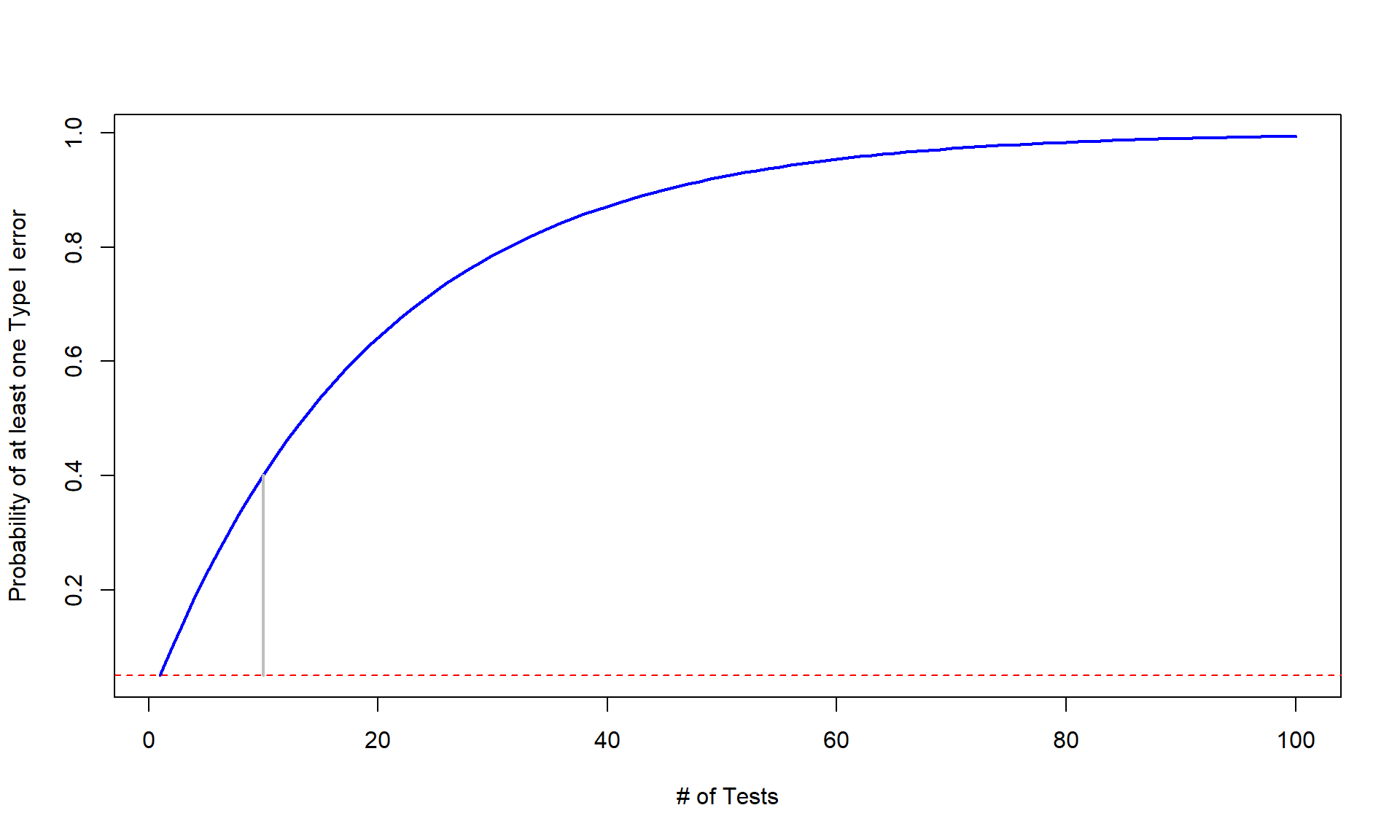
## 2      Min -5.136510 -2.6857436 1.24042295 2.736930 5.011190 0.03539750 2.874454 1000       0

Generally, the challenge in this situation is that if you perform many tests (ten were the focus before) at the same time (instead of just one test), you inflate the Type I error rate across the tests. We can define the family-wise error rate as the probability that at least one error is made on a set of tests or, more compactly, Pr(At least 1 error is made) where Pr() is the probability of an event occurring. The family-wise error is meant to capture the overall situation in terms of measuring the likelihood of making a mistake if we consider many tests, each with some chance of making their own mistake, and focus on how often we make at least one error when we do many tests. A quick probability calculation shows the magnitude of the problem. If we start with a 5% significance level test, then Pr(Type I error on one test) = 0.05 and the Pr(no errors made on one test) = 0.95, by definition. This is our standard hypothesis testing situation. Now, suppose we have \(m\) independent tests, then

\[\begin{array}{ll} & \text{Pr(make at least 1 Type I error given all null hypotheses are true)} \\ & = 1 - \text{Pr(no errors made)} \\ & = 1 - 0.95^m. \end{array}\]

Figure 2.20 shows how the probability of having at least one false detection grows rapidly with the number of tests, \(m\). The plot stops at 100 tests since it is effectively a 100% chance of at least one false detection. It might seem like doing 100 tests is a lot, but, as mentioned before, some researchers consider situations where millions of tests are considered. Researchers want to make sure that when they report a “significant” result that it is really likely to be a real result and will show up as a difference in the next data set they collect. Some researchers are now collecting multiple data sets to use in a single study and using one data set to identify interesting results and then using a validation or test data set that they withheld from initial analysis to try to verify that the first results are also present in that second data set. This also has problems but the only way to develop an understanding of a process is to look across a suite of studies and learn from that accumulation of evidence. This is a good start but needs to be coupled with complete reporting of all results, even those that have p-values larger than 0.05 to avoid the bias identified in the previous simulation study.

Figure 2.20: Plot of family-wise error rate (bold solid line) as the number of tests performed increases. Dashed line indicates 0.05 and grey solid line highlights the probability of at least on error on \(m = 10\) tests.

All hope is not lost when multiple tests are being considered in the same study or by a researcher and exploring more than one result need not lead to clearly biased and flawed results being reported. To account for multiple testing in the same study/analysis, there are many approaches that adjust results to acknowledge that multiple tests are being considered. A simple approach called the “Bonferroni Correction” (Bland and Altman 1995) is a good starting point for learning about these methods. It works to control the family-wise error rate of a suite of tests by either dividing \(\alpha\) by the number of tests (\(\alpha/m\)) or, equivalently and more usefully, multiplying the p-value by the number of tests being considered (\(p-value_{adjusted} = p-value \cdot m\) or \(1\) if \(p-value \cdot m > 1\)). The “Bonferroni adjusted p-values” are then used as regular p-values to assess evidence against each null hypothesis but now accounting for exploring many of them together. There are some assumptions that this adjustment method makes that make it to generally be a conservative adjustment method. In particular, it assumes that all \(m\) tests are independent of each other and that the null hypothesis was true for all \(m\) tests conducted. While all p-values should be reported in this situation when considering ten results, the impacts of using a Bonferroni correction are that the resulting p-values are not driving inflated Type I error rates even if the smallest p-value is the main focus of the results. The correction also provides a suggestion of decreasing evidence in the first test result because it is now incorporated in considering ten results instead of one.

The following code repeats the simulation study but with the p-values adjusted for multiple testing within each simulation but does not repeat tracking the estimated differences in the means as this is not impacted by the p-value adjustment process. The p.adjust function provides Bonferroni corrections to a vector of p-values (here ten are collected together) using the bonferroni method option (p.adjust(pval10, method = "bonferroni")) and then stores those results. Figure 2.21 shows the results for the first result and minimum result again, but now with these corrections incorporated. The plots may look a bit odd, but in the first data set, so many of the first data sets had p-values that were “large” that they were adjusted to have p-values of 1 (so no evidence against the null once we account for multiple testing). The distribution for the minimum p-value results with adjustment more closely resembles the distribution of the first result p-values from Figure 2.19, except for some minor clumping up at adjusted p-values of 1.

# Simulation study of generating 10 data sets and either using the first 
# or "best p-value" result:
set.seed(1234)

B <- 1000 # # of simulations
pvalues <- pvalues_Min <- matrix(NA, nrow = B) #To store results
for (b in (1:B)){ #Simulation study loop to repeat process B times
  # Create empty vectors to store 10 results for each b
  pval10 <- matrix(NA, nrow = 10) 
  for (c in (1:10)){ #Loop to create 10 data sets and extract results
    ddsub$SimDistance <- simulate(lm_commonmean)[[1]]
    # Estimate two group model using simulated responses
    lm_sim <- lm(SimDistance ~ Condition, data = ddsub) 
    pval10[c] <- summary(lm_sim)$coef[2,4]
  }
  
  pval10 <- p.adjust(pval10, method = "bonferroni")
  
  pvalues[b] <- pval10[1] #Store first result adjusted p-value
  
  pvalues_Min[b] <- min(pval10) #Store smallest adjusted p-value
}

# Put results together
results <- tibble(pvalue_results = c(pvalues, pvalues_Min), 
                  Scenario = rep(c("First", "Min"), each = B))

pirateplot(pvalue_results ~ Scenario, data = results, inf.f.o = 0, inf.b.o = 0,
           avg.line.o = 0, main = "P-value results")
abline(h = 0.05, lwd = 2, col = "red", lty = 2)

Figure 2.21: Pirate-plot of a simulation study results of p-values with Bonferroni correction.

By applying the pdata function to the two groups of results, we can directly assess how many of each type (“First” or “Min”) resulted in p-values less than 0.05. It ends up that if we adjust for ten tests and just focus on the first result, it is really hard to find moderate or strong evidence against the null hypothesis as only 3 in 1,000 results had adjusted p-values less than 0.05. When the focus is on the “best” (or minimum) p-value result when ten are considered and adjustments are made, 52 out of 1,000 results (0.052) show at least moderate evidence against the null hypothesis. This is the rate we would expect from a well-behaved hypothesis test when the null hypothesis is true – that we would only make a mistake 5% of the time when \(\alpha\) is 0.05.

# Numerical summaries of results
favstats(pvalue_results ~ Scenario, data = results)

##   Scenario         min        Q1  median Q3 max      mean        sd    n missing
## 1    First 0.017051496 1.0000000 1.00000  1   1 0.9628911 0.1502805 1000       0
## 2      Min 0.005727895 0.2718018 0.64637  1   1 0.6212932 0.3597701 1000       0

# Proportion of simulations with adjusted p-values less than 0.05
pdata(pvalue_results ~ Scenario, data = results, .05, lower.tail = T)

##   Scenario pdata_v
## 1    First   0.003
## 2      Min   0.052

So adjusting for multiple testing is suggested when multiple tests are being considered “simultaneously”. The Bonferroni adjustment is easy but also crude and can be conservative in applications, especially when the number of tests grows very large (think of multiplying all your p-values by \(m\) = 1,000,000). So other approaches are considered in situations with many tests (there are six other options in the p.adjust function and other functions for doing similar things in R) and there are other approaches that are customized for particular situations with one example discussed in Chapter 3. The biggest lesson as a statistics student to take from this is that all results are of interest and should be reported and that adjustment of p-values should be considered in studies where many results are being considered. If you are reading results that seem to have walked discretely around these issues you should be suspicious of the real strength of their evidence.

While it wasn’t used here, the same general code used to explore this multiple testing issue could be used to explore the power of a particular procedure. If simulations were created from a model with a difference in the means in the groups, then the null hypothesis would have been false and the rate of correctly rejecting the null hypothesis could be studied. The rate of correct rejections is the power of a procedure for a chosen version of a true alternative hypothesis (there are many ways to have it be true and you have to choose one to study power) and simply switching the model being simulated from would allow that to be explored. We could also use similar code to compare the power and Type I error rates of parametric versus permutation procedures or to explore situations where an assumption is not true. The steps would be similar – decide on what you need to simulate from and track a quantity of interest across repeated simulated data sets.