2.10: Bootstrap confidence intervals for difference in GPAs

We can now apply the new confidence interval methods on the STAT 217 grade data. This time we start with the parametric 95% confidence interval “by hand” in R and then use lm to verify our result. The favstats output provides us with the required information to calculate the confidence interval, with the estimated difference in the sample mean GPAs of \(3.338-3.0886 = 0.2494\):

favstats(GPA ~ Sex, data = s217)

##   Sex  min  Q1 median   Q3 max     mean        sd  n missing
## 1   F 2.50 3.1  3.400 3.70   4 3.338378 0.4074549 37       0
## 2   M 1.96 2.8  3.175 3.46   4 3.088571 0.4151789 42       0

The \(df\) are \(37+42-2 = 77\). Using the SDs from the two groups and their sample sizes, we can calculate \(s_p\):

sp <- sqrt(((37 - 1)*(0.4075^2) + (42 - 1)*(0.41518^2))/(37 + 42 - 2))
sp

## [1] 0.4116072

The margin of error is:

qt(0.975, df = 77)*sp*sqrt(1/37 + 1/42)

## [1] 0.1847982

All together, the 95% confidence interval is:

3.338 - 3.0886 + c(-1,1)*qt(0.975, df = 77)*sp*sqrt(1/37 + 1/42)

## [1] 0.0646018 0.4341982

So we are 95% confident that the difference in the true mean GPAs between females and males (females minus males) is between 0.065 and 0.434 GPA points. We get a similar result from confint on lm, except that lm switched the direction of the comparison from what was done “by hand” above, with the estimated mean difference of -0.25 GPA points (male - female) and similarly switched CI:

lm_GPA <- lm(GPA ~ Sex, data = s217)
summary(lm_GPA)

## 
## Call:
## lm(formula = GPA ~ Sex, data = s217)
## 
## Residuals:
##      Min       1Q   Median       3Q      Max 
## -1.12857 -0.28857  0.06162  0.36162  0.91143 
## 
## Coefficients:
##             Estimate Std. Error t value Pr(>|t|)
## (Intercept)  3.33838    0.06766  49.337  < 2e-16
## SexM        -0.24981    0.09280  -2.692  0.00871
## 
## Residual standard error: 0.4116 on 77 degrees of freedom
## Multiple R-squared:  0.08601,    Adjusted R-squared:  0.07414 
## F-statistic: 7.246 on 1 and 77 DF,  p-value: 0.008713

confint(lm_GPA)

##                  2.5 %      97.5 %
## (Intercept)  3.2036416  3.47311517
## SexM        -0.4345955 -0.06501838

Note that we can easily switch to 90% or 99% confidence intervals by simply changing the percentile in qt or changing the level option in the confint function.

qt(0.95, df = 77) #For 90% confidence and 77 df

## [1] 1.664885

qt(0.995, df = 77) #For 99% confidence and 77 df

## [1] 2.641198

confint(lm_GPA, level = 0.9) #90% confidence interval

##                    5 %        95 %
## (Intercept)  3.2257252  3.45103159
## SexM        -0.4043084 -0.09530553

confint(lm_GPA, level = 0.99) #99% confidence interval

##                  0.5 %       99.5 %
## (Intercept)  3.1596636  3.517093108
## SexM        -0.4949103 -0.004703598

As a review of some basic ideas with confidence intervals make sure you can answer the following questions:

1. What is the impact of increasing the confidence level in this situation?
2. What happens to the width of the confidence interval if the size of the SE increases or decreases?
3. What about increasing the sample size – should that increase or decrease the width of the interval?

All the general results you learned before about impacts to widths of CIs hold in this situation whether we are considering the parametric or bootstrap methods…

To finish this example, we will generate the comparable bootstrap 90% confidence interval using the bootstrap distribution in Figure 2.26.

Tobs <- coef(lm_GPA)[2]; Tobs

##       SexM 
## -0.2498069

B <- 1000
set.seed(1234)
Tstar <- matrix(NA, nrow = B)

for (b in (1:B)){
  lmP <- lm(GPA ~ Sex, data = resample(s217))
  Tstar[b] <- coef(lmP)[2]
}

quantiles <- qdata(Tstar, c(0.05, 0.95))
quantiles

##          5%         95% 
## -0.39290566 -0.09622185

The output tells us that the 90% confidence interval is from -0.393 to -0.096 GPA points. The bootstrap distribution with the observed difference in the sample means and these cut-offs is displayed in Figure 2.26 using this code:

Figure 2.26: Histogram and density curve of bootstrap distribution of difference in sample mean GPAs (male minus female) with observed difference (solid vertical line) and quantiles that delineate the 90% confidence intervals (dashed vertical lines).

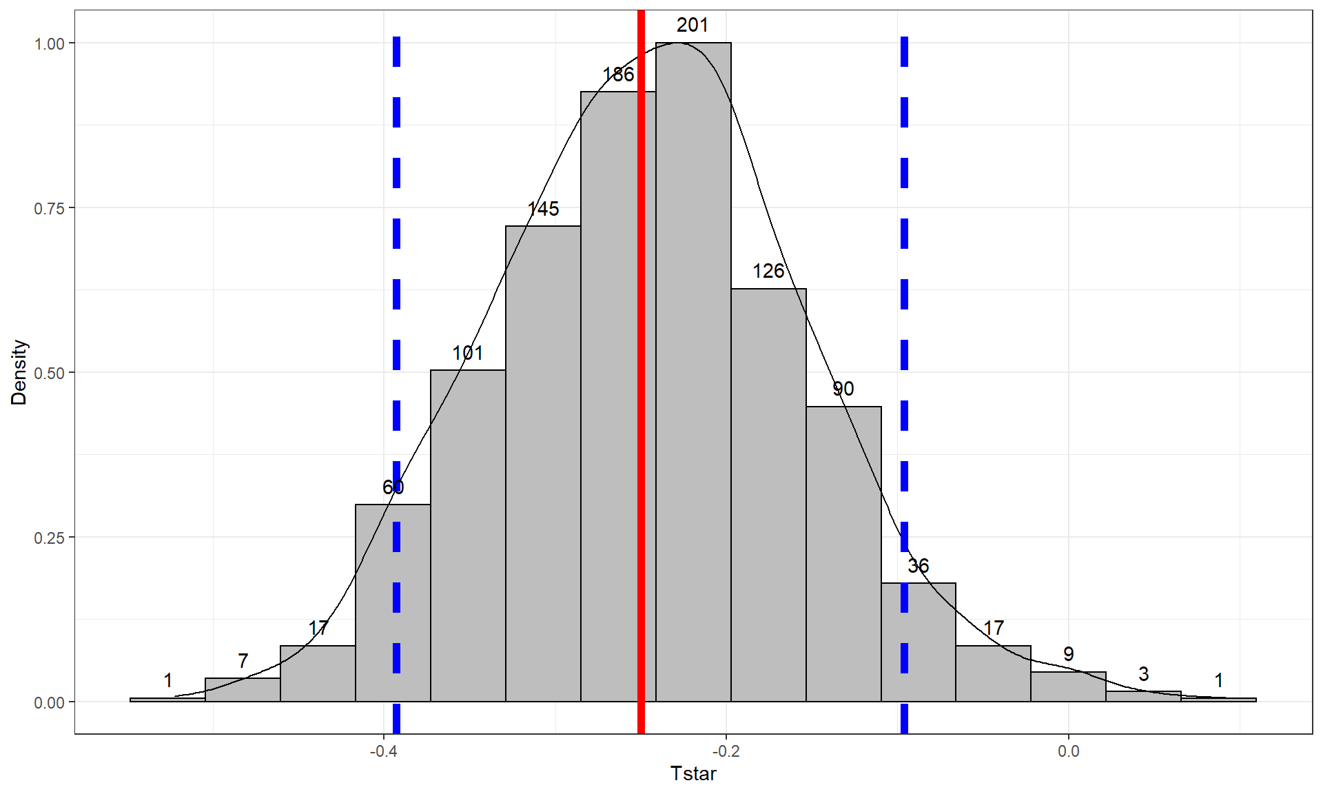
tibble(Tstar) %>% ggplot(aes(x = Tstar)) + 
  geom_histogram(aes(y = ..ncount..), bins = 15, col = 1, fill = "grey", 
                 center = 0) + 
  geom_density(aes(y = ..scaled..)) +
  theme_bw() +
  labs(y = "Density") +
  geom_vline(xintercept = quantiles, col = "blue", lwd = 2, lty = 2) + 
  geom_vline(xintercept = Tobs, col = "red", lwd = 2) +
  stat_bin(aes(y = ..ncount.., label = ..count..), bins = 15, 
           geom = "text", vjust = -0.75)

In the previous output, the parametric 90% confidence interval is from -0.404 to -0.095, suggesting similar results again from the two approaches. Based on the bootstrap CI, we can say that we are 90% confident that the difference in the true mean GPAs for STAT 217 students is between -0.393 to -0.096 GPA points (male minus females). This result would be usefully added to step 5 in the 6+ steps of the hypothesis testing protocol with an updated result of:

5. Report and discuss an estimate of the size of the differences, with confidence interval(s) if appropriate.
   • Females were estimated to have a higher mean GPA by 0.3 points (90% bootstrap confidence interval: 0.096 to 0.393). This difference of 0.3 on a GPA scale does not seem like a very large difference in the means even though we were able to detect a difference in the groups.

Throughout the text, pay attention to the distinctions between parameters and statistics, focusing on the differences between estimates based on the sample and inferences for the population of interest in the form of the parameters of interest. Remember that statistics are summaries of the sample information and parameters are characteristics of populations (which we rarely know). And that our inferences are limited to the population that we randomly sampled from, if we randomly sampled.