Unit 4B: Inference for Relationships

In the previous unit, we learned to perform inference for a single categorical or quantitative variable in the form of point estimation, confidence intervals or hypothesis testing.

The inference was actually

• about the population proportion (when the variable of interest was categorical) and
• about the population mean (when the variable of interest was quantitative).

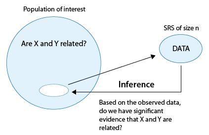
Our next (and final) goal for this course is to perform inference about relationships between two variables in a population, based on an observed relationship between variables in a sample. Here is what the process looks like:

We are interested in studying whether a relationship exists between the variables X and Y in a population of interest. We choose a random sample and collect data on both variables from the subjects.

Our goal is to determine whether these data provide strong enough evidence for us to generalize the observed relationship in the sample and conclude (with some acceptable and agreed-upon level of uncertainty) that a relationship between X and Y exists in the entire population.

The primary form of inference that we will use in this unit is hypothesis testing but we will discuss confidence intervals both to estimate unknown parameters of interest involving two variables and as an alternative way of determining the conclusion to our hypothesis test.

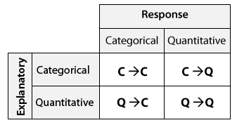
Recall that when we discussed examining the relationship between two variables in the Exploratory Data Analysis unit, our discussion was framed around the role-type classification. This part of the course will be structured exactly in the same way.

In other words, we will look at hypothesis testing in the 3 sections corresponding to cases C→Q, C→C, and Q→Q in the table below.

Recall that case Q→C is not specifically addressed in this course other than that we may investigate the association between these variables using the same methods as case C→Q.

It is also important to remember what we learned about lurking variables and causation.

• If our explanatory variable was part of a well-designed experiment then it may be possible for us to claim a causal effect

• But if it was based upon an observational study, we must be cautious to imply only a relationship or association between the two variables, not a direct causal link between the explanatory and response variable.

Unlike the previous part of the course on Inference for One Variable, where we discussed in some detail the theory behind the machinery of the test (such as the null distribution of the test statistic, under which the p-values are calculated), in the inferential procedures that we will introduce in Inference for Relationships, we will discuss much less of that kind of detail.

The principles are the same, but the details behind the null distribution of the test statistic (under which the p-value is calculated) become more complicated and require knowledge of theoretical results that are beyond the scope of this course.

Instead, within each of the inferential methods we will focus on:

• When the inferential method is appropriate for use.

• Under what conditions the procedure can safely be used.

• The conceptual idea behind the test (as it is usually captured by the test statistic).

• How to use software to carry out the procedure in order to get the p-value of the test.

• Interpreting the results in the context of the problem.

• Also, we will continue to introduce each test according to the four-step process of hypothesis testing.