Case C→Q

CO-4: Distinguish among different measurement scales, choose the appropriate descriptive and inferential statistical methods based on these distinctions, and interpret the results.

REVIEW: Unit 1 Case C-Q

Video

Video: Case C→Q (5:23)

Introduction

Recall the role-type classification table framing our discussion on inference about the relationship between two variables.

We start with case C→Q, where the explanatory variable is categorical and the response variable is quantitative.

Recall that in the Exploratory Data Analysis unit, examining the relationship between X and Y in this situation amounts, in practice, to:

• Comparing the distributions of the (quantitative) response Y for each value (category) of the explanatory X.

To do that, we used

• side-by-side boxplots (each representing the distribution of Y in one of the groups defined by X),
• and supplemented the display with the corresponding descriptive statistics.

We will need to add one layer of difficulty here with the possibility that we may have paired or matched samples as opposed to independent samples or groups. Note that all of the examples we discussed in Case CQ in Unit 1 consisted of independent samples.

First we will review the general scenario.

Comparing Means between Groups

To understand the logic, we’ll start with an example and then generalize.

EXAMPLE: GPA and Year in College

Suppose that our variable of interest is the GPA of college students in the United States. From Unint 4A, we know that since GPA is quantitative, we will conduct inference on μ, the (population) mean GPA among all U.S. college students.

Since this section is about relationships, let’s assume that what we are really interested in is not simply GPA, but the relationship between:

• X : year in college (1 = freshmen, 2 = sophomore, 3 = junior, 4 = senior) and
• Y : GPA

In other words, we want to explore whether GPA is related to year in college.

The way to think about this is that the population of U.S. college students is now broken into 4 sub-populations: freshmen, sophomores, juniors and seniors. Within each of these four groups, we are interested in the GPA.

The inference must therefore involve the 4 sub-population means:

• μ₁ : mean GPA among freshmen in the United States.
• μ₂ : mean GPA among sophomores in the United States
• μ₃ : mean GPA among juniors in the United States
• μ₄ : mean GPA among seniors in the United States

It makes sense that the inference about the relationship between year and GPA has to be based on some kind of comparison of these four means.

If we infer that these four means are not all equal (i.e., that there are some differences in GPA across years in college) then that’s equivalent to saying GPA is related to year in college. Let’s summarize this example with a figure:

In general, making inferences about the relationship between X and Y in Case C→Q boils down to comparing the means of Y in the sub-populations, which are created by the categories defined by X (say k categories). The following figure summarizes this:

We will split this into two different scenarios (k = 2 and k > 2), where k is the number of categories defined by X.

For example:

• If we are interested in whether GPA (Y) is related to gender (X), this is a scenario where k = 2 (since gender has only two categories: M, F), and the inference will boil down to comparing the mean GPA in the sub-population of males to that in the sub-population of females.

• On the other hand, in the example we looked at earlier, the relationship between GPA (Y) and year in college (X) is a scenario where k > 2 or more specifically, k = 4 (since year has four categories).

Caution

In terms of inference, these two situations (k = 2 and k > 2) will be treated differently!

Scenario with k = 2

Scenario with k > 2

2. This large population is broken up into k sub-populations, each with its own mean μ. To infer on relationship between Y and X, we'll need to compare these k means." height="459" loading="lazy" src="http://phhp-faculty-cantrell.sites.m...7/image013.gif" title="The entire population is represented by a large circle, for which we wonder if there is a relationship between Y and X. k > 2. This large population is broken up into k sub-populations, each with its own mean μ. To infer on relationship between Y and X, we'll need to compare these k means." width="565">

Dependent vs. Independent Samples (k = 2)

Learning Objectives

LO 4.37: Identify and distinquish between independent and dependent samples.

Furthermore, within the scenario of comparing two means (i.e., examining the relationship between X and Y, when X has only two categories, k = 2) we will distinguish between two scenarios.

Here, the distinction is somewhat subtle, and has to do with how the samples from each of the two sub-populations we’re comparing are chosen. In other words, it depends upon what type of study design will be implemented.

We have learned that many experiments, as well as observational studies, make a comparison between two groups (sub-populations) defined by the categories of the explanatory variable (X), in order to see if the response (Y) differs.

In some situations, one group (sub-population 1) is defined by one category of X, and another independent group (sub-population 2) is defined by the other category of X. Independent samples are then taken from each group for comparison.

EXAMPLE:

Suppose we are conducting a clinical trial. Participants are randomized into two independent subpopulations:

• those who are given a drug and
• those who are given a placebo.

Each individual appears in only one of these two groups and individuals are not matched or paired in any way. Thus the two samples or groups are independent. We can say those given the drug are independent from those given the placebo.

Recall: By randomly assigning individuals to the treatment we control for both known and unknown lurking variables.

EXAMPLE:

Suppose the Highway Patrol wants to study the reaction times of drivers with a blood alcohol content of half the legal limit in their state.

An observational study was designed which would also serve as publicity on the topic of drinking and driving. At a large event where enough alcohol would be consumed to obtain plenty of potential study participants, officers set up an obstacle course and provided the vehicles. (Other considerations were also implemented to keep the car and track conditions consistent for each participant.)

Volunteers were recruited from those in attendance and given a breathalyzer test to determine their blood alcohol content. Two types of volunteers were chosen to participate:

• Those with a blood alcohol content of zero – as measured by the breathalyzer – of which 10 were chosen to drive the course.
• Those with a blood alcohol content within a small range of half the legal limit (in Florida this would be around 0.04%) – of which 9 were chosen.

Here also, we have two independent groups – even if originally they were taken from the same sample of volunteers – each individual appears in only one of the two groups, the comparison of the reaction times is a comparison between two independent groups.

However, in this study, there was NO random assignment to the treatment and so we would need to be much more concerned about the possibility of lurking variables in this study compared to one in which individuals were randomized into one of these two groups.

We will see it may be more appropriate in some studies to use the same individual as a subject in BOTH treatments – this will result in dependent samples.

When a matched pairs sample design is used, each observation in one sample is matched/paired/linked with an observation in the other sample. These are sometimes called “dependent samples.”

Matching could be by person (if the same person is measured twice), or could actually be a pair of individuals who belong together in a relevant way (husband and wife, siblings).

In this design, then, the same individual or a matched pair of individuals is used to make two measurements of the response – one for each of the two levels of the categorical explanatory variable.

Advantages of a paired sample approach include:

• Reduced measurement error since the variance within subjects is typically smaller than that between subjects
• Requires smaller number of subjects to achieve the same power than independent sample methods.

Disadvantages of a paired sample approach include:

• An order effect based upon which treatment individuals received first.
• A carryover effect such as a drug remaining in the system.
• Testing effect such as particpants learning the obstacle course in the first run improving their performance in the 2nd.

EXAMPLE:

Suppose we are conducting a study on a pain blocker which can be applied to the skin and are comparing two different dosage levels of the solution which in this study will be applied to the forearm.

For each participant both solutions are applied with the following protocol:

• Which drug is applied to which arm is random.
• Patients and clinical staff are blind to the two treatment applications.
• Pain tolerance is measured on both arms using the same standard test with the order of testing randomized.

Here we have dependent samples since the same patient appears in both dosage groups.

Again, randomization is employed to help minimize other issues related to study design such as an order or testing effect.

EXAMPLE:

Suppose the department of motor vehicles wants to check whether drivers are impaired after drinking two beers.

The reaction times (measured in seconds) in an obstacle course are measured for 8 randomly selected drivers before and then after the consumption of two beers.

We have a matched-pairs design, since each individual was measured twice, once before and once after.

In matched pairs, the comparison between the reaction times is done for each individual.

Comment:

• Note that in the first figure, where the samples are independent, the sample sizes of the two independent samples need not be the same.

• On the other hand, it is obvious from the design that in the matched pairs the sample sizes of the two samples must be the same (and thus we used n for both).

• Dependent samples can occur in many other settings but for now we focus on the case of investigating the relationship between a two-level categorical explanatory variable and a quantitative response variable.

Let’s Summarize:

We will begin our discussion of Inference for Relationships with Case C-Q, where the explanatory variable (X) is categorical and the response variable (Y) is quantitative. We discussed that inference in this case amounts to comparing population means.

• We distinguish between scenarios where the explanatory variable (X) has only two categories and scenarios wheret he explanatory variable (X) has MORE than two categories.

• When comparing two means, we make the futher distinction between situations where we have independent samples and those where we have matched pairs.

• For comparing more than two means in this course, we will focus only on the situation where we have independent samples. In studies with more than two groups on dependent samples, it is good to know that a common method used is repeated measures but we will not cover it here.

• We will first discuss comparing two population means starting with matched pairs (dependent samples) then independent samples and conclude with comparing more than two population means in the case of independent samples.

Now test your skills at identifying the three scenarios in Case C-Q.

Did I Get This?: Scenarios in Case C-Q
(Non-Interactive Version – Spoiler Alert)

Looking Ahead – Methods in Case C-Q

• Methods in BOLD will be our main focus in this unit.

Here is a summary of the tests we will learn for the scenario where k = 2.

Independent Samples (More Emphasis)	Dependent Samples (Less Emphasis)
Standard Tests Two Sample T-Test Assuming Equal Variances Two Sample T-Test Assuming Unequal Variances Non-Parametric Test Mann-Whitney U (or Wilcoxon Rank-Sum) Test	Standard Test Paired T-Test Non-Parametric Tests Sign Test Wilcoxon Signed-Rank Test

Here is a summary of the tests we will learn for the scenario where k > 2.

Independent Samples (Only Emphasis)	Dependent Samples (Not Discussed)
Standard Tests One-way ANOVA (Analysis of Variance) Non-Parametric Test Kruskal–Wallis One-way ANOVA	Standard Test Repeated Measures ANOVA (or similar)

Paired Samples

Caution

As we mentioned at the end of the Introduction to Unit 4B, we will focus only on two-sided tests for the remainder of this course. One-sided tests are often possible but rarely used in clinical research.

• Introduction – Matched Pairs (Paired t-test)
• The Idea Behind the Paired t-Test
• Test Procedure for Paired T-Test
• Example: Drinking and Driving
• Example: IQ Scores
• Additional Data for Practice
• Non-Parametric Tests
• Let’s Summarize

CO-4: Distinguish among different measurement scales, choose the appropriate descriptive and inferential statistical methods based on these distinctions, and interpret the results.

Learning Objectives

LO 4.35: For a data analysis situation involving two variables, choose the appropriate inferential method for examining the relationship between the variables and justify the choice.

Learning Objectives

LO 4.36: For a data analysis situation involving two variables, carry out the appropriate inferential method for examining relationships between the variables and draw the correct conclusions in context.

CO-5: Determine preferred methodological alternatives to commonly used statistical methods when assumptions are not met.

Video

Video: Paired Samples (27:19)

Related SAS Tutorials

• 8B (2:55) EDA of Differences
• 8C (5:20) Paired T-Test and Non Parametric Tests

Related SPSS Tutorials

• 8B (2:00) EDA of Differences
• 8C (3:11) Paired T-Test
• 8D (3:32) Non Parametric (Paired)

Introduction – Matched Pairs (Paired t-test)

Learning Objectives

LO 4.37: Identify and distinguish between independent and dependent samples.

Learning Objectives

LO 4.38: In a given context, determine the appropriate standard method for comparing groups and provide the correct conclusions given the appropriate software output.

Learning Objectives

LO 4.39: In a given context, set up the appropriate null and alternative hypotheses for comparing groups.

We are in Case CQ of inference about relationships, where the explanatory variable is categorical and the response variable is quantitative.

As we mentioned in the summary of the introduction to Case C→Q, the first case that we will deal with is that involving matched pairs. In this case:

• The samples are paired or matched. Every observation in one sample is linked with an observation in the other sample.

• In other words, the samples are dependent.

Notice from this point forward we will use the terms population 1 and population 2 instead of sub-population 1 and sub-population 2. Either terminology is correct.

One of the most common cases where dependent samples occur is when both samples have the same subjects and they are “paired by subject.” In other words, each subject is measured twice on the response variable, typically before and then after some kind of treatment/intervention in order to assess its effectiveness.

EXAMPLE: SAT Prep Class

Suppose you want to assess the effectiveness of an SAT prep class.

It would make sense to use the matched pairs design and record each sampled student’s SAT score before and after the SAT prep classes are attended:

Recall that the two populations represent the two values of the explanatory variable. In this situation, those two values come from a single set of subjects.

• In other words, both populations really have the same students.
• However, each population has a different value of the explanatory variable. Those values are: no prep class, prep class.

This, however, is not the only case where the paired design is used. Other cases are when the pairs are “natural pairs,” such as siblings, twins, or couples.

Notes about graphical summaries for paired data in Case CQ:

• Due to the paired nature of this type of data, we cannot really use side-by-side boxplots to visualize this data as the information contained in the pairing is completely lost.
• We will need to provide graphical summaries of the differences themselves in order to explore this type of data.

The Idea Behind Paired t-Test

The idea behind the paired t-test is to reduce this two-sample situation, where we are comparing two means, to a single sample situation where we are doing inference on a single mean, and then use a simple t-test that we introduced in the previous module.

In this setting, we can easily reduce the raw data to a set of differences and conduct a one-sample t-test.

• Thus we simplify our inference procedure to a problem where we are making an inference about a single mean: the mean of the differences.

In other words, by reducing the two samples to one sample of differences, we are essentially reducing the problem from a problem where we’re comparing two means (i.e., doing inference on μ₁−μ₂) to a problem in which we are studying one mean.

In general, in every matched pairs problem, our data consist of 2 samples which are organized in n pairs:

We reduce the two samples to only one by calculating the difference between the two observations for each pair.

For example, think of Sample 1 as “before” and Sample 2 as “after”. We can find the difference between the before and after results for each participant, which gives us only one sample, namely “before – after”. We label this difference as “d” in the illustration below.

The paired t-test is based on this one sample of n differences,

and it uses those differences as data for a one-sample t-test on a single mean — the mean of the differences.

This is the general idea behind the paired t-test; it is nothing more than a regular one-sample t-test for the mean of the differences!

Test Procedure for Paired T-Test

We will now go through the 4-step process of the paired t-test.

• Step 1: State the hypotheses

Recall that in the t-test for a single mean our null hypothesis was: Ho: μ = μ₀ and the alternative was one of Ha: μ < μ₀ or μ > μ₀ or μ ≠ μ₀. Since the paired t-test is a special case of the one-sample t-test, the hypotheses are the same except that:

Instead of simply μ we use the notation μ_d to denote that the parameter of interest is the mean of the differences.

In this course our null value μ₀ is always 0. In other words, going back to our original paired samples our null hypothesis claims that that there is no difference between the two means. (Technically, it does not have to be zero if you are interested in a more specific difference – for example, you might be interested in showing that there is a reduction in blood pressure of more than 10 points but we will not specifically look at such situations).

Therefore, in the paired t-test: The null hypothesis is always:

Ho: μ_d = 0
(There IS NO association between the categorical explanatory variable and the quantitative response variable)

We will focus on the two-sided alternative hypothesis of the form:

Ha: μ_d ≠ 0
(There IS AN association between the categorical explanatory variable and the quantitative response variable)

Some students find it helpful to know that it turns out that μ_d = μ₁ – μ₂ (in other words, the difference between the means is the same as the mean of the differences). You may find it easier to first think about the hypotheses in terms of μ₁ – μ₂ and then represent it in terms of μ_d.

Did I Get This? Setting up Hypotheses
(Non-Interactive Version – Spoiler Alert)

• Step 2: Obtain data, check conditions, and summarize data

The paired t-test, as a special case of a one-sample t-test, can be safely used as long as:

The sample of differences is random (or at least can be considered random in context).

The distribution of the differences in the population should vary normally if you have small samples. If the sample size is large, it is safe to use the paired t-test regardless of whether the differences vary normally or not. This condition is satisfied in the three situations marked by a green check mark in the table below.

Note: normality is checked by looking at the histogram of differences, and as long as no clear violation of normality (such as extreme skewness and/or outliers) is apparent, the normality assumption is reasonable.

Assuming that we can safely use the paired t-test, the data are summarized by a test statistic:

\(t = \dfrac{\bar{y}_d - 0}{s_d / \sqrt{n}}\)

where

\(\bar{y}_d = \text{ sample mean of the differences}\)

\(s_d = \text{sample standard deviation of the differences}\)

This test statistic measures (in standard errors) how far our data are (represented by the sample mean of the differences) from the null hypothesis (represented by the null value, 0).

Notice this test statistic has the same general form as those discussed earlier:

\(\text{test statistic} = \dfrac{\text{estimator - null value}}{\text{standard error of estimator}}\)

• Step 3: Find the p-value of the test by using the test statistic as follows

As a special case of the one-sample t-test, the null distribution of the paired t-test statistic is a t distribution (with n – 1 degrees of freedom), which is the distribution under which the p-values are calculated. We will use software to find the p-value for us.

• Step 4: Conclusion

As usual, we draw our conclusion based on the p-value. Be sure to write your conclusions in context by specifying your current variables and/or precisely describing the population mean difference in terms of the current variables.

In particular, if a cutoff probability, α (significance level), is specified, we reject Ho if the p-value is less than α. Otherwise, we fail to reject Ho.

If the p-value is small, there is a statistically significant difference between what was observed in the sample and what was claimed in Ho, so we reject Ho.

Conclusion: There is enough evidence that the categorical explanatory variable is associated with the quantitative response variable. More specifically, there is enough evidence that the population mean difference is not equal to zero.

Remember: a small p-value tells us that there is very little chance of getting data like those observed (or even more extreme) if the null hypothesis were true. Therefore, a small p-value indicates that we should reject the null hypothesis.

If the p-value is not small, we do not have enough statistical evidence to reject Ho.

Conclusion: There is NOT enough evidence that the categorical explanatory variable is associated with the quantitative response variable. More specifically, there is NOT enough evidence that the population mean difference is not equal to zero.

Notice how much better the first sentence sounds! It can get difficult to correctly phrase these conclusions in terms of the mean difference without confusing double negatives.

Learning Objectives

LO 4.40: Based upon the output for a paired t-test, correctly interpret in context the appropriate confidence interval for the population mean-difference.

As in previous methods, we can follow-up with a confidence interval for the mean difference, μ_d and interpret this interval in the context of the problem.

Interpretation: We are 95% confident that the population mean difference (described in context) is between (lower bound) and (upper bound).

Confidence intervals can also be used to determine whether or not to reject the null hypothesis of the test based upon whether or not the null value of zero falls outside the interval or inside.

If the null value, 0, falls outside the confidence interval, Ho is rejected. (Zero is NOT a plausible value based upon the confidence interval)

If the null value, 0, falls inside the confidence interval, Ho is not rejected. (Zero IS a plausible value based upon the confidence interval)

NOTE: Be careful to choose the correct confidence interval about the population mean difference and not the individual confidence intervals for the means in the groups themselves.

Now let’s look at an example.

EXAMPLE: Drinking and Driving

Note: In some of the videos presented in the course materials, we do conduct the one-sided test for this data instead of the two-sided test we conduct below. In Unit 4B we are going to restrict our attention to two-sided tests supplemented by confidence intervals as needed to provide more information about the effect of interest.

• Here is the SPSS Output for this example as well as the SAS Output and SAS Code.

Drunk driving is one of the main causes of car accidents. Interviews with drunk drivers who were involved in accidents and survived revealed that one of the main problems is that drivers do not realize that they are impaired, thinking “I only had 1-2 drinks … I am OK to drive.”

A sample of 20 drivers was chosen, and their reaction times in an obstacle course were measured before and after drinking two beers. The purpose of this study was to check whether drivers are impaired after drinking two beers. Here is a figure summarizing this study:

• Note that the categorical explanatory variable here is “drinking 2 beers (Yes/No)”, and the quantitative response variable is the reaction time.

• By using the matched pairs design in this study (i.e., by measuring each driver twice), the researchers isolated the effect of the two beers on the drivers and eliminated any other confounding factors that might influence the reaction times (such as the driver’s experience, age, etc.).

• For each driver, the two measurements are the total reaction time before drinking two beers, and after. You can see the data by following the links in Step 2 below.

Since the measurements are paired, we can easily reduce the raw data to a set of differences and conduct a one-sample t-test.

Here are some of the results for this data:

Step 1: State the hypotheses

We define μ_d = the population mean difference in reaction times (Before – After).

As we mentioned, the null hypothesis is:

• Ho: μ_d = 0 (indicating that the population of the differences are centered at a number that IS ZERO)

The null hypothesis claims that the differences in reaction times are centered at (or around) 0, indicating that drinking two beers has no real impact on reaction times. In other words, drivers are not impaired after drinking two beers.

Although we really want to know whether their reaction times are longer after the two beers, we will still focus on conducting two-sided hypothesis tests. We will be able to address whether the reaction times are longer after two beers when we look at the confidence interval.

Therefore, we will use the two-sided alternative:

• Ha: μ_d ≠ 0 (indicating that the population of the differences are centered at a number that is NOT ZERO)

Step 2: Obtain data, check conditions, and summarize data

• Data: Beers SPSS format, SAS format, Excel format, CSV format

Let’s first check whether we can safely proceed with the paired t-test, by checking the two conditions.

• The sample of drivers was chosen at random.

• The sample size is not large (n = 20), so in order to proceed, we need to look at the histogram or QQ-plot of the differences and make sure there is no evidence that the normality assumption is not met.

We can see from the histogram above that there is no evidence of violation of the normality assumption (on the contrary, the histogram looks quite normal).

Also note that the vast majority of the differences are negative (i.e., the total reaction times for most of the drivers are larger after the two beers), suggesting that the data provide evidence against the null hypothesis.

The question (which the p-value will answer) is whether these data provide strong enough evidence or not against the null hypothesis. We can safely proceed to calculate the test statistic (which in practice we leave to the software to calculate for us).

Test Statistic: We will use software to calculate the test statistic which is t = -2.58.

• Recall: This indicates that the data (represented by the sample mean of the differences) are 2.58 standard errors below the null hypothesis (represented by the null value, 0).

Step 3: Find the p-value of the test by using the test statistic as follows

As a special case of the one-sample t-test, the null distribution of the paired t-test statistic is a t distribution (with n – 1 degrees of freedom), which is the distribution under which the p-values are calculated.

We will let the software find the p-value for us, and in this case, gives us a p-value of 0.0183 (SAS) or 0.018 (SPSS).

The small p-value tells us that there is very little chance of getting data like those observed (or even more extreme) if the null hypothesis were true. More specifically, there is less than a 2% chance (0.018=1.8%) of obtaining a test statistic of -2.58 (or lower) or 2.58 (or higher), assuming that 2 beers have no impact on reaction times.

Step 4: Conclusion

In our example, the p-value is 0.018, indicating that the data provide enough evidence to reject Ho.

• Conclusion: There is enough evidence that drinking two beers is associated with differences in reaction times of drivers.

Follow-up Confidence Interval:

As a follow-up to this conclusion, we quantify the effect that two beers have on the driver, using the 95% confidence interval for μ_d.

Using statistical software, we find that the 95% confidence interval for μ_d, the mean of the differences (before – after), is roughly (-0.9, -0.1).

Note: Since the differences were calculated before-after, longer reaction times after the beers would translate into negative differences.

• Interpretation: We are 95% confident that after drinking two beers, the true mean increase in total reaction time of drivers is between 0.1 and 0.9 of a second.

• Thus, the results of the study do indicate impairment of drivers (longer reaction times) not the other way around!

Since the confidence interval does not contain the null value of zero, we can use it to decide to reject the null hypothesis. Zero is not a plausible value of the population mean difference based upon the confidence interval. Notice that using this method is not always practical as often we still need to provide the p-value in clinical research. (Note: this is NOT the interpretation of the confidence interval but a method of using the confidence interval to conduct a hypothesis test.)

Did I Get This? Confidence Intervals for the Population Mean Difference
(Non-Interactive Version – Spoiler Alert)

Practical Significance:

We should definitely ask ourselves if this is practically significant and I would argue that it is.

• Although a difference in the mean reaction time of 0.1 second might not be too bad, a difference of 0.9 seconds is likely a problem.

• Even at a difference in reaction time of 0.4 seconds, if you were traveling 60 miles per hour, this would translate into a distance traveled of around 35 feet.

Many Students Wonder: One-sided vs. Two-sided P-values

In the output, we are generally provided the two-sided p-value. We must be very careful when converting this to a one-sided p-value (if this is not provided by the software)

• IF the data are in the direction of our alternative hypothesis then we can simply take half of the two-sided p-value.

• IF, however, the data are NOT in the direction of the alternative, the correct p-value is VERY LARGE and is the complement of (one minus) half the two-sided p-value.

The “driving after having 2 beers” example is a case in which observations are paired by subject. In other words, both samples have the same subject, so that each subject is measured twice. Typically, as in our example, one of the measurements occurs before a treatment/intervention (2 beers in our case), and the other measurement after the treatment/intervention.

Our next example is another typical type of study where the matched pairs design is used—it is a study involving twins.

EXAMPLE: IQ Scores

Researchers have long been interested in the extent to which intelligence, as measured by IQ score, is affected by “nurture” as opposed to “nature”: that is, are people’s IQ scores mainly a result of their upbringing and environment, or are they mainly an inherited trait?

A study was designed to measure the effect of home environment on intelligence, or more specifically, the study was designed to address the question: “Are there statistically significant differences in IQ scores between people who were raised by their birth parents, and those who were raised by someone else?”

In order to be able to answer this question, the researchers needed to get two groups of subjects (one from the population of people who were raised by their birth parents, and one from the population of people who were raised by someone else) who are as similar as possible in all other respects. In particular, since genetic differences may also affect intelligence, the researchers wanted to control for this confounding factor.

We know from our discussion on study design (in the Producing Data unit of the course) that one way to (at least theoretically) control for all confounding factors is randomization—randomizing subjects to the different treatment groups. In this case, however, this is not possible. This is an observational study; you cannot randomize children to either be raised by their birth parents or to be raised by someone else. How else can we eliminate the genetics factor? We can conduct a “twin study.”

Because identical twins are genetically the same, a good design for obtaining information to answer this question would be to compare IQ scores for identical twins, one of whom is raised by birth parents and the other by someone else. Such a design (matched pairs) is an excellent way of making a comparison between individuals who only differ with respect to the explanatory variable of interest (upbringing) but are as alike as they can possibly be in all other important aspects (inborn intelligence). Identical twins raised apart were studied by Susan Farber, who published her studies in the book “Identical Twins Reared Apart” (1981, Basic Books).

In this problem, we are going to use the data that appear in Farber’s book in table E6, of the IQ scores of 32 pairs of identical twins who were reared apart.

Here is a figure that will help you understand this study:

Here are the important things to note in the figure:

• We are essentially comparing the mean IQ scores in two populations that are defined by our (two-valued categorical) explanatory variable — upbringing (X), whose two values are: raised by birth parents, raised by someone else.

• This is a matched pairs design (as opposed to a two independent samples design), since each observation in one sample is linked (matched) with an observation in the second sample. The observations are paired by twins.

Each of the 32 rows represents one pair of twins. Keeping the notation that we used above, twin 1 is the twin that was raised by his/her birth parents, and twin 2 is the twin that was raised by someone else. Let’s carry out the analysis.

Step 1: State the hypotheses

Recall that in matched pairs, we reduce the data from two samples to one sample of differences:

The hypotheses are stated in terms of the mean of the difference where, μ_d = population mean difference in IQ scores (Birth Parents – Someone Else):

• Ho: μ_d = 0 (indicating that the population of the differences are centered at a number that IS ZERO)

• Ha: μ_d ≠ 0 (indicating that the population of the differences are centered at a number that is NOT ZERO)

Step 2: Obtain data, check conditions, and summarize data

Is it safe to use the paired t-test in this case?

• Clearly, the samples of twins are not random samples from the two populations. However, in this context, they can be considered as random, assuming that there is nothing special about the IQ of a person just because he/she has an identical twin.

• The sample size here is n = 32. Even though it’s the case that if we use the n > 30 rule of thumb our sample can be considered large, it is sort of a borderline case, so just to be on the safe side, we should look at the histogram of the differences just to make sure that we do not see anything extreme. (Comment: Looking at the histogram of differences in every case is useful even if the sample is very large, just in order to get a sense of the data. Recall: “Always look at the data.”)

The data don’t reveal anything that we should be worried about (like very extreme skewness or outliers), so we can safely proceed. Looking at the histogram, we note that most of the differences are negative, indicating that in most of the 32 pairs of twins, twin 2 (raised by someone else) has a higher IQ.

From this point we rely on statistical software, and find that:

• t-value = -1.85
• p-value = 0.074

Our test statistic is -1.85.

Our data (represented by the sample mean of the differences) are 1.85 standard errors below the null hypothesis (represented by the null value 0).

Step 3: Find the p-value of the test by using the test statistic as follows

The p-value is 0.074, indicating that there is a 7.4% chance of obtaining data like those observed (or even more extreme) assuming that H_o is true (i.e., assuming that there are no differences in IQ scores between people who were raised by their natural parents and those who weren’t).

Step 4: Conclusion

Using the conventional significance level (cut-off probability) of .05, our p-value is not small enough, and we therefore cannot reject H_o.

• Conclusion: Our data do not provide enough evidence to conclude that whether a person was raised by his/her natural parents has an impact on the person’s intelligence (as measured by IQ scores).

Confidence Interval:

The 95% confidence interval for the population mean difference is (-6.11322, 0.30072).

Interpretation:

• We are 95% confident that the population mean IQ for twins raised by someone else is between 6.11 greater to 0.3 lower than that for twins raised by their birth parents.

• OR … We are 95% confident that the population mean IQ for twins raised by their birth parents is between 6.11 lower to 0.3 greater than that for twins raised by someone else.

• Note: The order of the groups as well as the numbers provided in the interval can vary, what is important is to get the “lower” and “greater” with the correct value based upon the group order being used.
  • Here we used Birth Parents – Someone Else and thus a positive number for our population mean difference indicates that birth parents group is higher (someone else gorup is lower) and a negative number indicates the someone else group is higher (birth parents group is lower).

This confidence interval does contain zero and thus results in the same conclusion to the hypothesis test. Zero IS a plausible value of the population mean difference and thus we cannot reject the null hypothesis.

Practical Significance:

• The confidence interval does “lean” towards the difference being negative, indicating that in most of the 32 pairs of twins, twin 2 (raised by someone else) has a higher IQ. The sample mean difference is -2.9 so we would need to consider whether this value and range of plausible values have any real practical significance.

• In this case, I don’t think I would consider a difference in IQ score of around 3 points to be very important in practice (but others could reasonably disagree).

It is very important to pay attention to whether the two-sample t-test or the paired t-test is appropriate. In other words, being aware of the study design is extremely important. Consider our example, if we had not “caught” that this is a matched pairs design, and had analyzed the data as if the two samples were independent using the two-sample t-test, we would have obtained a p-value of 0.114.

Note that using this (wrong) method to analyze the data, and a significance level of 0.05, we would conclude that the data do not provide enough evidence for us to conclude that reaction times differed after drinking two beers. This is an example of how using the wrong statistical method can lead you to wrong conclusions, which in this context can have very serious implications.

Comments:

• The 95% confidence interval for μ can be used here in the same way as for proportions to conduct the two-sided test (checking whether the null value falls inside or outside the confidence interval) or following a t-test where Ho was rejected to get insight into the value of μ.

• In most situations in practice we use two-sided hypothesis tests, followed by confidence intervals to gain more insight.

Now try a complete example for yourself.

Learn By Doing: Matched Pairs – Gosset’s Seed Data
(Non-Interactive Version – Spoiler Alert)

Additional Data for Practice

Here are two other datasets with paired samples.

• Seeds: SPSS format, SAS format, Excel format, CSV format
• Twins: SPSS format, SAS format, Excel format, CSV format

Non-Parametric Alternatives for Matched Pair Data

Learning Objectives

LO 5.1: For a data analysis situation involving two variables, determine the appropriate alternative (non-parametric) method when assumptions of our standard methods are not met.

The statistical tests we have previously discussed (and many we will discuss) require assumptions about the distribution in the population or about the requirements to use a certain approximation as the sampling distribution. These methods are called parametric.

When these assumptions are not valid, alternative methods often exist to test similar hypotheses. Tests which require only minimal distributional assumptions, if any, are called non-parametric or distribution-free tests.

At the end of this section we will provide some details (see Details for Non-Parametric Alternatives), for now we simply want to mention that there are two common non-parametric alternatives to the paired t-test. They are:

• Sign Test
• Wilcoxon Signed-Rank Test

The fact that both of these tests have the word “sign” in them is not a coincidence – it is due to the fact that we will be interested in whether the differences have a positive sign or a negative sign – and the fact that this word appears in both of these tests can help you to remember that they correspond to paired methods where we are often interested in whether there was an increase (positive sign) or a decrease (negative sign).

Let’s Summarize

• The paired t-test is used to compare two population means when the two samples (drawn from the two populations) are dependent in the sense that every observation in one sample can be linked to an observation in the other sample. Such a design is called “matched pairs.”

• The most common case in which the matched pairs design is used is when the same subjects are measured twice, usually before and then after some kind of treatment and/or intervention. Another classic case are studies involving twins.

• In the background, we have a two-valued categorical explanatory whose categories define the two populations we are comparing and whose effect on the response variable we are trying to assess.

• The idea behind the paired t-test is to reduce the data from two samples to just one sample of the differences, and use these observed differences as data for inference about a single mean — the mean of the differences, μ_d.

• The paired t-test is therefore simply a one-sample t-test for the mean of the differences μ_d, where the null value is 0.

• Once we verify that we can safely proceed with the paired t-test, we use software output to carry it out.

• A 95% confidence interval for μ_d can be very insightful after a test has rejected the null hypothesis, and can also be used for testing in the two-sided case.

• Two non-parametric alternatives to the paired t-test are the sign test and the Wilcoxon signed–rank test. (See Details for Non-Parametric Alternatives.)

Two Independent Samples

CO-4: Distinguish among different measurement scales, choose the appropriate descriptive and inferential statistical methods based on these distinctions, and interpret the results

Learning Objectives

LO 4.35: For a data analysis situation involving two variables, choose the appropriate inferential method for examining the relationship between the variables and justify the choice.

Learning Objectives

LO 4.36: For a data analysis situation involving two variables, carry out the appropriate inferential method for examining relationships between the variables and draw the correct conclusions in context.

CO-5: Determine preferred methodological alternatives to commonly used statistical methods when assumptions are not met.

REVIEW: Unit 1 Case C-Q

Video

Video: Two Independent Samples (38:56)

Related SAS Tutorials

• 7A (2:32) Numeric Summaries by Groups
• 7B (3:03) Side-By-Side Boxplots
• 7C (6:57) Two Sample T-Test

Related SPSS Tutorials

• 7A (3:29) Numeric Summaries by Groups
• 7B (1:59) Side-By-Side Boxplots
• 7C (5:30) Two Sample T-Test

Introduction

Here is a summary of the tests we will learn for the scenario where k = 2. Methods in BOLD will be our main focus.

We have completed our discussion on dependent samples (2nd column) and now we move on to independent samples (1st column).

Independent Samples (More Emphasis)	Dependent Samples (Less Emphasis)
Standard Tests Two Sample T-Test Assuming Equal Variances Two Sample T-Test Assuming Unequal Variances Non-Parametric Test Mann-Whitney U (or Wilcoxon Rank-Sum) Test	Standard Test Paired T-Test Non-Parametric Tests Sign Test Wilcoxon Signed-Rank Test

Dependent vs. Independent Samples

Learning Objectives

LO 4.37: Identify and distinguish between independent and dependent samples.

We have discussed the dependent sample case where observations are matched/paired/linked between the two samples. Recall that in that scenario observations can be the same individual or two individuals who are matched between samples. To analyze data from dependent samples, we simply took the differences and analyzed the difference using one-sample techniques.

Now we will discuss the independent sample case. In this case, all individuals are independent of all other individuals in their sample as well as all individuals in the other sample. This is most often accomplished by either:

• Taking a random sample from each of the two groups under study. For example to compare heights of males and females, we could take a random sample of 100 females and another random sample of 100 males. The result would be two samples which are independent of each other.

• Taking a random sample from the entire population and then dividing it into two sub-samples based upon the grouping variable of interest. For example, we take a random sample of U.S. adults and then split them into two samples based upon gender. This results in a sub-sample of females and a sub-sample of males which are independent of each other.

Comparing Two Means – Two Independent Samples T-test

Learning Objectives

LO 4.38: In a given context, determine the appropriate standard method for comparing groups and provide the correct conclusions given the appropriate software output.

Learning Objectives

LO 4.39: In a given context, set up the appropriate null and alternative hypotheses for comparing groups.

Recall that here we are interested in the effect of a two-valued (k = 2) categorical variable (X) on a quantitative response (Y). Random samples from the two sub-populations (defined by the two categories of X) are obtained and we need to evaluate whether or not the data provide enough evidence for us to believe that the two sub-population means are different.

In other words, our goal is to test whether the means μ₁ and μ₂ (which are the means of the variable of interest in the two sub-populations) are equal or not, and in order to do that we have two samples, one from each sub-population, which were chosen independently of each other.

The test that we will learn here is commonly known as the two-sample t-test. As the name suggests, this is a t-test, which as we know means that the p-values for this test are calculated under some t-distribution.

Here are figures that illustrate some of the examples we will cover. Notice how the original variables X (categorical variable with two levels) and Y (quantitative variable) are represented. Think about the fact that we are in case C → Q!

As in our discussion of dependent samples, we will often simplify our terminology and simply use the terms “population 1” and “population 2” instead of referring to these as sub-populations. Either terminology is fine.

Many Students Wonder: Two Independent Samples

Question: Does it matter which population we label as population 1 and which as population 2?

Answer: No, it does not matter as long as you are consistent, meaning that you do not switch labels in the middle.

• BUT… considering how you label the populations is important in stating the hypotheses and in the interpretation of the results.

Steps for the Two-Sample T-test

Recall that our goal is to compare the means μ₁ and μ₂ based on the two independent samples.

• Step 1: State the hypotheses

The hypotheses represent our goal to compare μ₁and μ₂.

The null hypothesis is always:

Ho: μ₁ – μ₂ = 0 (which is the same as μ₁ = μ₂)
(There IS NO association between the categorical explanatory variable and the quantitative response variable)

We will focus on the two-sided alternative hypothesis of the form:

Ha: μ₁ – μ₂ ≠ 0 (which is the same as μ₁ ≠ μ₂) (two-sided)
(There IS AN association between the categorical explanatory variable and the quantitative response variable)

Note that the null hypothesis claims that there is no difference between the means. Conceptually, Ho claims that there is no relationship between the two relevant variables (X and Y).

Our parameter of interest in this case (the parameter about which we are making an inference) is the difference between the means (μ₁ – μ₂) and the null value is 0. The alternative hypothesis claims that there is a difference between the means.

Did I Get This? What do our hypotheses mean in context?
(Non-Interactive Version – Spoiler Alert)

• Step 2: Obtain data, check conditions, and summarize data

The two-sample t-test can be safely used as long as the following conditions are met:

The two samples are indeed independent.

We are in one of the following two scenarios:

(i) Both populations are normal, or more specifically, the distribution of the response Y in both populations is normal, and both samples are random (or at least can be considered as such). In practice, checking normality in the populations is done by looking at each of the samples using a histogram and checking whether there are any signs that the populations are not normal. Such signs could be extreme skewness and/or extreme outliers.

(ii) The populations are known or discovered not to be normal, but the sample size of each of the random samples is large enough (we can use the rule of thumb that a sample size greater than 30 is considered large enough).

Did I Get This? Conditions for Two Independent Samples
(Non-Interactive Version – Spoiler Alert)

Assuming that we can safely use the two-sample t-test, we need to summarize the data, and in particular, calculate our data summary—the test statistic.

Test Statistic for Two-Sample T-test:

There are two choices for our test statistic, and we must choose the appropriate one to summarize our data We will see how to choose between the two test statistics in the next section. The two options are as follows:

We use the following notation to describe our samples:

\(n_1, n_2\) = sample sizes of the samples from population 1 and population 2

\(\bar{y}_1, \bar{y}_2\) = sample means of the samples from population 1 and population 2

\(s_1, s_2\) = sample standard deviations of the samples from population 1 and population 2

\(s_p\) = pooled estimate of a common population standard deviation

Here are the two cases for our test statistic.

(A) Equal Variances: If it is safe to assume that the two populations have equal standard deviations, we can pool our estimates of this common population standard deviation and use the following test statistic.

\(t=\dfrac{\bar{y}_{1}-\bar{y}_{2}-0}{s_{p} \sqrt{\frac{1}{n_{1}}+\frac{1}{n_{2}}}}\)

where

\(s_{p}=\sqrt{\dfrac{\left(n_{1}-1\right) s_{1}^{2}+\left(n_{2}-1\right) s_{2}^{2}}{n_{1}+n_{2}-2}}\)

(B) Unequal Variances: If it is NOT safe to assume that the two populations have equal standard deviations, we have unequal standard deviations and must use the following test statistic.

\(t=\dfrac{\bar{y}_{1}-\bar{y}_{2}-0}{\sqrt{\frac{s_{1}^{2}}{n_{1}}+\frac{s_{2}^{2}}{n_{2}}}}\)

Comments:

• It is possible to never assume equal variances; however, if the assumption of equal variances is satisfied the equal variances t-test will have greater power to detect the difference of interest.

• We will not be calculating the values of these test statistics by hand in this course. We will instead rely on software to obtain the value for us.

• Both of these test statistics measure (in standard errors) how far our data are (represented by the difference of the sample means) from the null hypothesis (represented by the null value, 0).

• These test statistics have the same general form as others we have discussed. We will not discuss the derivation of the standard errors in each case but you should understand this general form and be able to identify each component for a specific test statistic.

\(\text{test statistic} = \dfrac{\text{estimator - null value}}{\text{standard error of estimator}}\)

• Step 3: Find the p-value of the test by using the test statistic as follows

Each of these tests rely on a particular t-distribution under which the p-values are calculated. In the case where equal variances are assumed, the degrees of freedom are simply:

\(n_1 + n_2 - 2\)

whereas in the case of unequal variances, the formula for the degrees of freedom is more complex. We will rely on the software to obtain the degrees of freedom in both cases and provided us with the correct p-value (usually this will be a two-sided p-value).

• Step 4: Conclusion

As usual, we draw our conclusion based on the p-value. Be sure to write your conclusions in context by specifying your current variables and/or precisely describing the difference in population means in terms of the current variables.

If the p-value is small, there is a statistically significant difference between what was observed in the sample and what was claimed in Ho, so we reject Ho.

Conclusion: There is enough evidence that the categorical explanatory variable is related to (or associated with) the quantitative response variable. More specifically, there is enough evidence that the difference in population means is not equal to zero.

If the p-value is not small, we do not have enough statistical evidence to reject Ho.

Conclusion: There is NOT enough evidence that the categorical explanatory variable is related to (or associated with) the quantitative response variable. More specifically, there is enough evidence that the difference in population means is not equal to zero.

In particular, if a cutoff probability, α (significance level), is specified, we reject Ho if the p-value is less than α. Otherwise, we do not reject Ho.

Learning Objectives

LO 4.41: Based upon the output for a two-sample t-test, correctly interpret in context the appropriate confidence interval for the difference between population means

As in previous methods, we can follow-up with a confidence interval for the difference between population means, μ₁ – μ₂ and interpret this interval in the context of the problem.

Interpretation: We are 95% confident that the population mean for (one group) is between __________________ compared to the population mean for (the other group).

Confidence intervals can also be used to determine whether or not to reject the null hypothesis of the test based upon whether or not the null value of zero falls outside the interval or inside.

If the null value, 0, falls outside the confidence interval, Ho is rejected. (Zero is NOT a plausible value based upon the confidence interval)

If the null value, 0, falls inside the confidence interval, Ho is not rejected. (Zero IS a plausible value based upon the confidence interval)

NOTE: Be careful to choose the correct confidence interval about the difference between population means using the same assumption (variances equal or variances unequal) and not the individual confidence intervals for the means in the groups themselves.

Many Students Wonder: Reading Statistical Software Output for Two-Sample T-test

Test for Equality of Variances (or Standard Deviations)

Learning Objectives

LO 4.42: Based upon the output for a two-sample t-test, determine whether to use the results assuming equal variances or those assuming unequal variances.

Since we have two possible tests we can conduct, based upon whether or not we can assume the population standard deviations (or variances) are equal, we need a method to determine which test to use.

Although you can make a reasonable guess using information from the data (i.e. look at the distributions and estimates of the standard deviations and see if you feel they are reasonably equal), we have a test which can help us here, called the test for Equality of Variances. This output is automatically displayed in many software packages when a two-sample t-test is requested although the particular test used may vary.The hypotheses of this test are:

Ho: σ₁ = σ₂ (the standard deviations in the two populations are the same)

Ha: σ₁ ≠ σ₂ (the standard deviations in the two populations are not the same)

• If the p-value of this test for equal variances is small, there is enough evidence that the standard deviations in the two populations are different and we cannot assume equal variances.
  • IMPORTANT! In this case, when we conduct the two-sample t-test to compare the population means, we use the test statistic for unequal variances.
• If the p-value of this test is large, there is not enough evidence that the standard deviations in the two populations are different. In this case we will assume equal variances since we have no clear evidence to the contrary.
  • IMPORTANT! In this case, when we conduct the two-sample t-test to compare the population means, we use the test statistic for equal variances.

Now let’s look at a complete example of conducting a two-sample t-test, including the embedded test for equality of variances.

EXAMPLE: What is more important - personality or looks?

This question was asked of a random sample of 239 college students, who were to answer on a scale of 1 to 25. An answer of 1 means personality has maximum importance and looks no importance at all, whereas an answer of 25 means looks have maximum importance and personality no importance at all. The purpose of this survey was to examine whether males and females differ with respect to the importance of looks vs. personality.

Note that the data have the following format:

Score (Y)	Gender (X)
15	Male
13	Female
10	Female
12	Male
14	Female
14	Male
6	Male
17	Male
etc.

The format of the data reminds us that we are essentially examining the relationship between the two-valued categorical variable, gender, and the quantitative response, score. The two values of the categorical explanatory variable (k = 2) define the two populations that we are comparing — males and females. The comparison is with respect to the response variable score. Here is a figure that summarizes the example:

Comments:

• Note that this figure emphasizes how the fact that our explanatory is a two-valued categorical variable means that in practice we are comparing two populations (defined by these two values) with respect to our response Y.

• Note that even though the problem description just says that we had 239 students, the figure tells us that there were 85 males in the sample, and 150 females.

• Following up on comment 2, note that 85 + 150 = 235 and not 239. In these data (which are real) there are four “missing observations,” 4 students for which we do not have the value of the response variable, “importance.” This could be due to a number of reasons, such as recording error or non response. The bottom line is that even though data were collected from 239 students, effectively we have data from only 235. (Recommended: Go through the data file and note that there are 4 cases of missing observations: students 34, 138, 179, and 183).

Step 1: State the hypotheses

Recall that the purpose of this survey was to examine whether the opinions of females and males differ with respect to the importance of looks vs. personality. The hypotheses in this case are therefore:

Ho: μ₁ – μ₂ = 0 (which is the same as μ₁ = μ₂)

Ha: μ₁ – μ₂ ≠ 0 (which is the same as μ₁ ≠ μ₂)

where μ₁ represents the mean “looks vs personality score” for females and μ₂ represents the mean “looks vs personality score” for males.

It is important to understand that conceptually, the two hypotheses claim:

Ho: Score (of looks vs. personality) is not related to gender

Ha: Score (of looks vs. personality) is related to gender

Step 2: Obtain data, check conditions, and summarize data

• Data: Looks SPSS format, SAS format, Excel format, CSV format
• Let’s first check whether the conditions that allow us to safely use the two-sample t-test are met.
  • Here, 239 students were chosen and were naturally divided into a sample of females and a sample of males. Since the students were chosen at random, the sample of females is independent of the sample of males.
  • Here we are in the second scenario — the sample sizes (150 and 85), are definitely large enough, and so we can proceed regardless of whether the populations are normal or not.
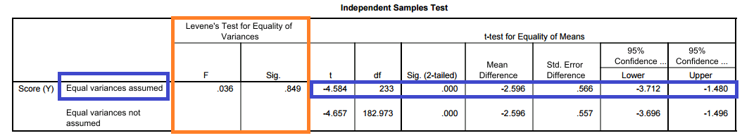
• In the output below we first look at the test for equality of variances (outlined in orange). The two-sample t-test results we will use are outlined in blue.
• There are TWO TESTS represented in this output and we must make the correct decision for BOTH of these tests to correctly proceed.
• SOFTWARE OUTPUT In SPSS:
  • The p-value for the test of equality of variances is reported as 0.849 in the SIG column under Levene’s test for equality of variances. (Note this differs from the p-value found using SAS, two different tests are used by default between the two programs).
  • So we fail to reject the null hypothesis that the variances, or equivalently the standard deviations, are equal (Ho: σ₁ = σ₂).
  • Conclusion to test for equality of variances: We cannot conclude there is a difference in the variance of looks vs. personality score between males and females.
  • This results in using the row for Equal variances assumed to find the t-test results including the test statistic, p-value, and confidence interval for the difference. (Outlined in BLUE)

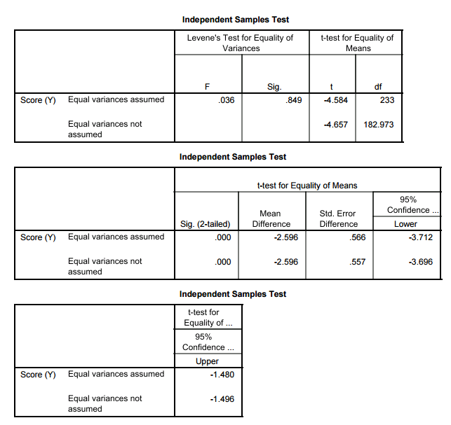
The output might also be broken up if you export or copy the items in certain ways. The results are the same but it can be more difficult to read.

• SOFTWARE OUTPUT In SAS:
  • The p-value for the test of equality of variances is reported as 0.5698 in the Pr > F column under equality of variances. (Note this differs from the p-value found using SPSS, two different tests are used by default between the two programs).
  • So we fail to reject the null hypothesis that the variances, or equivalently the standard deviations, are equal (Ho: σ₁ = σ₂).
  • Conclusion to test for equality of variances: We cannot conclude there is a difference in the variance of looks vs. personality score between males and females.
  • This results in using the row for POOLED method where equal variances are assumed to find the t-test results including the test statistic, p-value, and confidence interval for the difference. (Outlined in BLUE)

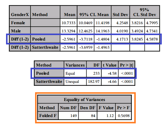
• TEST STATISTIC for Two-Sample T-test: In all of the results above, we determine that we will use the test which assumes the variances are EQUAL, and we find our test statistic of t = -4.58.

Step 3: Find the p-value of the test by using the test statistic as follows

• We will let the software find the p-value for us, and in this case, the p-value is less than our significance level of 0.05 in fact it is practically 0.
• This is found in SPSS in the equal variances assumed row under t-test in the SIG. (two-tailed) column given as 0.000 and in SAS in the POOLED ROW under Pr > |t| column given as <0.0001.
• A p-value which is practically 0 means that it would be almost impossible to get data like that observed (or even more extreme) had the null hypothesis been true.
• More specifically, in our example, if there were no differences between females and males with respect to whether they value looks vs. personality, it would be almost impossible (probability approximately 0) to get data where the difference between the sample means of females and males is -2.6 (that difference is 10.73 – 13.33 = -2.6) or more extreme.
• Comment: Note that the output tells us that the difference μ₁ – μ₂ is approximately -2.6. But more importantly, we want to know if this difference is statistically significant. To answer this, we use the fact that this difference is 4.58 standard errors below the null value.

Step 4: Conclusion

As usual a small p-value provides evidence against Ho. In our case our p-value is practically 0 (which is smaller than any level of significance that we will choose). The data therefore provide very strong evidence against Ho so we reject it.

• Conclusion: There is enough evidence that the mean Importance score (of looks vs personality) of males differs from that of females. In other words, males and females differ with respect to how they value looks vs. personality.

As a follow-up to this conclusion, we can construct a confidence interval for the difference between population means. In this case we will construct a confidence interval for μ₁ – μ₂ the population mean “looks vs personality score” for females minus the population mean “looks vs personality score” for males.

• Using statistical software, we find that the 95% confidence interval for μ₁ – μ₂ is roughly (-3.7, -1.5).
• This is found in SPSS in the equal variances assumed row under 95% confidence interval columns given as -3.712 to -1.480 and in SAS in the POOLED ROW under 95% CL MEAN column given as -3.7118 to -1.4804 (be careful NOT to choose the confidence interval for the standard deviation in the last column, 9% CL Std Dev).
• Interpretation:
  • We are 95% confident that the population mean “looks vs personality score” for females is between 3.7 and 1.5 points lower than that of males.
  • OR
  • We are 95% confident that the population mean “looks vs personality score” for males is between 3.7 and 1.5 points higher than that of females.
• The confidence interval therefore quantifies the effect that the explanatory variable (gender) has on the response (looks vs personality score).
• Since low values correspond to personality being more important and high values correspond to looks being more important, the result of our investigation suggests that, on average, females place personality higher than do males. Alternatively we could say that males place looks higher than do females.
• Note: The confidence interval does not contain zero (both values are negative based upon how we chose our groups) and thus using the confidence interval we can reject the null hypothesis here.

Practical Significance:

We should definitely ask ourselves if this is practically significant

• Is a true difference in population means as represented by our estimate from this data meaningful here? I will let you consider and answer for yourself.

SPSS Output for this example (Non-Parametric Output for Examples 1 and 2)

SAS Output and SAS Code (Includes Non-Parametric Test)

Here is another example.

EXAMPLE: BMI vs. Gender in Heart Attack Patients

A study was conducted which enrolled and followed heart attack patients in a certain metropolitan area. In this example we are interested in determining if there is a relationship between Body Mass Index (BMI) and gender. Individuals presenting to the hospital with a heart attack were randomly selected to participate in the study.

Step 1: State the hypotheses

Ho: μ₁ – μ₂ = 0 (which is the same as μ₁ = μ₂)

Ha: μ₁ – μ₂ ≠ 0 (which is the same as μ₁ ≠ μ₂)

where μ₁ represents the mean BMI for males and μ₂ represents the mean BMI for females.

It is important to understand that conceptually, the two hypotheses claim:

Ho: BMI is not related to gender in heart attack patients

Ha: BMI is related to gender in heart attack patients

Step 2: Obtain data, check conditions, and summarize data

• Data: WHAS500 SPSS format, SAS format
• Let’s first check whether the conditions that allow us to safely use the two-sample t-test are met.
  • Here, subjects were chosen and were naturally divided into a sample of females and a sample of males. Since the subjects were chosen at random, the sample of females is independent of the sample of males.
  • Here, we are in the second scenario — the sample sizes are extremely large, and so we can proceed regardless of whether the populations are normal or not.
• In the output below we first look at the test for equality of variances (outlined in orange). The two-sample t-test results we will use are outlined in blue.
• There are TWO TESTS represented in this output and we must make the correct decision for BOTH of these tests to correctly proceed.
• SOFTWARE OUTPUT In SPSS:
  • The p-value for the test of equality of variances is reported as 0.001 in the SIG column under Levene’s test for equality of variances.
  • So we reject the null hypothesis that the variances, or equivalently the standard deviations, are equal (Ho: σ₁ = σ₂).
  • Conclusion to test for equality of variances: We conclude there is enought evidence of a difference in the variance of looks vs. personality score between males and females.
  • This results in using the row for Equal variances NOT assumed to find the t-test results including the test statistic, p-value, and confidence interval for the difference. (Outlined in BLUE)

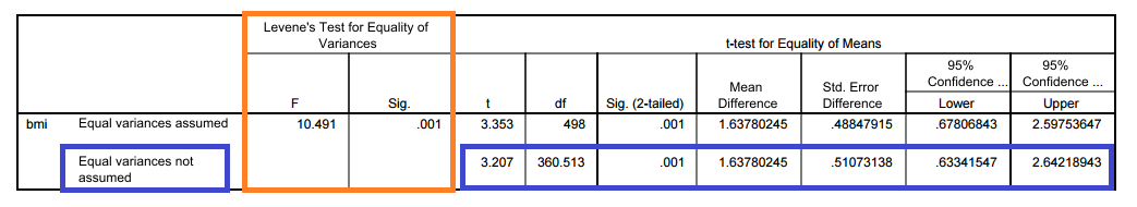
• SOFTWARE OUTPUT In SAS:
  • The p-value for the test of equality of variances is reported as 0.0004 in the Pr > F column under equality of variances.
  • So we reject the null hypothesis that the variances, or equivalently the standard deviations, are equal (Ho: σ₁ = σ₂).
  • Conclusion to test for equality of variances: We conclude there is enough evidence of a difference in the variance of looks vs. personality score between males and females.
  • This results in using the row for SATTERTHWAITE method where UNEQUAL variances are assumed to find the t-test results including the test statistic, p-value, and confidence interval for the difference. (Outlined in BLUE)

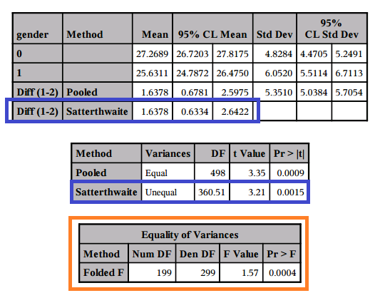
• TEST STATISTIC for Two-Sample T-test: In all of the results above, we determine that we will use the test which assumes the variances are UNEQUAL, and we find our test statistic of t = 3.21.

Step 3: Find the p-value of the test by using the test statistic as follows

• We will let the software find the p-value for us, and in this case, the p-value is less than our significance level of 0.05.
• This is found in SPSS in the UNEQUAL variances assumed row under t-test in the SIG. (two-tailed) column given as 0.001 and in SAS in the SATTERTHWAITE ROW under Pr > |t| column given as 0.0015.
• This p-value means that it would be extremely rare to get data like that observed (or even more extreme) had the null hypothesis been true.
• More specifically, in our example, if there were no differences between females and males with respect to BMI, it would be almost highly unlikely (0.001 probability) to get data where the difference between the sample mean BMIs of males and females is 1.64 or more extreme.
• Comment: Note that the output tells us that the difference μ₁ – μ₂ is approximately 1.64. But more importantly, we want to know if this difference is statistically significant. To answer this, we use the fact that this difference is 3.21 standard errors above the null value.

Step 4: Conclusion

As usual a small p-value provides evidence against Ho. In our case our p-value is 0.001 (which is smaller than any level of significance that we will choose). The data therefore provide very strong evidence against Ho so we reject it.

• Conclusion: The mean BMI of males differs from that of females. In other words, males and females differ with respect to BMI among heart attack patients.

As a follow-up to this conclusion, we can construct a confidence interval for the difference between population means. In this case we will construct a confidence interval for μ₁ – μ₂ the population mean BMI for males minus the population mean BMI for females.

• Using statistical software, we find that the 95% confidence interval for μ₁ – μ₂ is roughly (0.63, 2.64).
• This is found in SPSS in the UNEQUAL variances assumed row under 95% confidence interval columns and in SAS in the SATTERTHWAITE ROW under 95% CL MEAN column.
• Interpretation:
  • With 95% confidence that the population mean BMI for males is between 0.63 and 2.64 units larger than that of females.
  • OR
  • With 95% confidence that the population mean BMI for females is between 0.63 and 2.64 units smaller than that of males.

• The confidence interval therefore quantifies the effect of the explanatory variable (gender) on the response (BMI). Notice that we cannot imply a causal effect of gender on BMI based upon this result alone as there could be many lurking variables, unaccounted for in this analysis, which might be partially or even completely responsible for this difference.
• Note: The confidence interval does not contain zero (both values are positive based upon how we chose our groups) and thus using the confidence interval we can reject the null hypothesis here.

Practical Significance:

• We should definitely ask ourselves if this is practically significant
• Is a true difference in population means as represented by our estimate from this data meaningful here? Is a difference in BMI of between 0.53 and 2.64 of interest?
• I will let you consider and answer for yourself.

SPSS Output for this example (Non-Parametric Output for Examples 1 and 2)

SAS Output and SAS Code (Includes Non-Parametric Test)
Note: In the SAS output the variable gender is not formatted, in this case Males = 0 and Females = 1.

Comments:

You might ask yourself: “Where do we use the test statistic?”

It is true that for all practical purposes all we have to do is check that the conditions which allow us to use the two-sample t-test are met, lift the p-value from the output, and draw our conclusions accordingly.

However, we feel that it is important to mention the test statistic for two reasons:

• The test statistic is what’s behind the scenes; based on its null distribution and its value, the p-value is calculated.

• Apart from being the key for calculating the p-value, the test statistic is also itself a measure of the evidence stored in the data against Ho. As we mentioned, it measures (in standard errors) how different our data is from what is claimed in the null hypothesis.

Now try some more activities for yourself.

Did I Get This? Two-Sample T-test and Related Confidence Interval
(Non-Interactive Version – Spoiler Alert)

Non-Parametric Alternative: Wilcoxon Rank-Sum Test (Mann-Whitney U)

Learning Objectives

LO 5.1: For a data analysis situation involving two variables, determine the appropriate alternative (non-parametric) method when assumptions of our standard methods are not met.

We will look at one non-parametric test in the two-independent samples setting. More details will be discussed later (Details for Non-Parametric Alternatives).

• The Wilcoxon rank-sum test (Mann-Whitney U test) is a general test to compare two distributions in independent samples. It is a commonly used alternative to the two-sample t-test when the assumptions are not met.

k > 2 Independent Samples

CO-4: Distinguish among different measurement scales, choose the appropriate descriptive and inferential statistical methods based on these distinctions, and interpret the results.

Learning Objectives

LO 4.35: For a data analysis situation involving two variables, choose the appropriate inferential method for examining the relationship between the variables and justify the choice.

Learning Objectives

LO 4.36: For a data analysis situation involving two variables, carry out the appropriate inferential method for examining relationships between the variables and draw the correct conclusions in context.

CO-5: Determine preferred methodological alternatives to commonly used statistical methods when assumptions are not met.

REVIEW: Unit 1 Case C-Q

Video

Video: 2 Independent Samples">k > 2 Independent Samples (21:15)

Related SAS Tutorials

• 7A (2:32) Numeric Summaries by Groups
• 7B (3:03) Side-By-Side Boxplots
• 7D (4:07) One Way ANOVA

Related SPSS Tutorials

• 7A (3:29) Numeric Summaries by Groups
• 7B (1:59) Side-By-Side Boxplots
• 7D (4:22) One Way ANOVA

Introduction

In this part, we continue to handle situations involving one categorical explanatory variable and one quantitative response variable, which is case C→Q.

Here is a summary of the tests we have covered for the case where k = 2. Methods in BOLD are our main focus in this unit.

So far we have discussed the two samples and matched pairs designs, in which the categorical explanatory variable is two-valued. As we saw, in these cases, examining the relationship between the explanatory and the response variables amounts to comparing the mean of the response variable (Y) in two populations, which are defined by the two values of the explanatory variable (X). The difference between the two samples and matched pairs designs is that in the former, the two samples are independent, and in the latter, the samples are dependent.

Independent Samples (More Emphasis)	Dependent Samples (Less Emphasis)
Standard Tests Two Sample T-Test Assuming Equal Variances Two Sample T-Test Assuming Unequal Variances Non-Parametric Test Mann-Whitney U (or Wilcoxon Rank-Sum) Test	Standard Test Paired T-Test Non-Parametric Tests Sign Test Wilcoxon Signed-Rank Test

We now move on to the case where k > 2 when we have independent samples. Here is a summary of the tests we will learn for the case where k > 2. Notice we will not cover the dependent samples case in this course.

Independent Samples (Only Emphasis)	Dependent Samples (Not Discussed)
Standard Tests One-way ANOVA (Analysis of Variance) Non-Parametric Test Kruskal–Wallis One-way ANOVA	Standard Test Repeated Measures ANOVA (or similar)

Here, as in the two-valued case, making inferences about the relationship between the explanatory (X) and the response (Y) variables amounts to comparing the means of the response variable in the populations defined by the values of the explanatory variable, where the number of means we are comparing depends, of course, on the number of values of X.

Unlike the two-valued case, where we looked at two sub-cases (1) when the samples are independent (two samples design) and (2) when the samples are dependent (matched pairs design, here, we are just going to discuss the case where the samples are independent. In other words, we are just going to extend the two samples design to more than two independent samples.

The inferential method for comparing more than two means that we will introduce in this part is called ANalysis Of VAriance (abbreviated as ANOVA), and the test associated with this method is called the ANOVA F-test.

In most software, the data need to be arranged so that each row contains one observation with one variable recording X and another variable recording Y for each observation.

Comparing Two or More Means – The ANOVA F-test

Learning Objectives

LO 4.38: In a given context, determine the appropriate standard method for comparing groups and provide the correct conclusions given the appropriate software output.

Learning Objectives

LO 4.39: In a given context, set up the appropriate null and alternative hypotheses for comparing groups.

As we mentioned earlier, the test that we will present is called the ANOVA F-test, and as you’ll see, this test is different in two ways from all the tests we have presented so far:

• Unlike the previous tests, where we had three possible alternative hypotheses to choose from (depending on the context of the problem), in the ANOVA F-test there is only one alternative, which actually makes life simpler.

• The test statistic will not have the same structure as the test statistics we’ve seen so far. In other words, it will not have the form:

\(\text{test statistic} = \dfrac{\text{estimator - null value}}{\text{standard error of estimator}}\)

but a different structure that captures the essence of the F-test, and clarifies where the name “analysis of variance” is coming from.

What is the idea behind comparing more than two means?

The question we need to answer is: Are the differences among the sample means due to true differences among the μ’s (alternative hypothesis), or merely due to sampling variability or random chance (null hypothesis)?

---

Here are two sets of boxplots representing two possible scenarios:

Scenario #1

• Because of the large amount of spread within the groups, this data shows boxplots with plenty of overlap.
• One could imagine the data arising from 4 random samples taken from 4 populations, all having the same mean of about 11 or 12.
• The first group of values may have been a bit on the low side, and the other three a bit on the high side, but such differences could conceivably have come about by chance.
• This would be the case if the null hypothesis, claiming equal population means, were true.

---

Scenario #2

• Because of the small amount of spread within the groups, this data shows boxplots with very little overlap.
• It would be very hard to believe that we are sampling from four groups that have equal population means.
• This would be the case if the null hypothesis, claiming equal population means, were false.

---

Thus, in the language of hypothesis tests, we would say that if the data were configured as they are in scenario 1, we would not reject the null hypothesis that population means were equal for the k groups.

If the data were configured as they are in scenario 2, we would reject the null hypothesis, and we would conclude that not all population means are the same for the k groups.

Let’s summarize what we learned from this.

• The question we need to answer is: Are the differences among the sample means due to true differences among the μ’s (alternative hypothesis), or merely due to sampling variability (null hypothesis)?

In order to answer this question using data, we need to look at the variation among the sample means, but this alone is not enough.

We need to look at the variation among the sample means relative to the variation within the groups. In other words, we need to look at the quantity:

which measures to what extent the difference among the sample means for our groups dominates over the usual variation within sampled groups (which reflects differences in individuals that are typical in random samples).

When the variation within groups is large (like in scenario 1), the variation (differences) among the sample means may become negligible resulting in data which provide very little evidence against Ho. When the variation within groups is small (like in scenario 2), the variation among the sample means dominates over it, and the data have stronger evidence against Ho.

It has a different structure from all the test statistics we’ve looked at so far, but it is similar in that it is still a measure of the evidence against H₀. The larger F is (which happens when the denominator, the variation within groups, is small relative to the numerator, the variation among the sample means), the more evidence we have against H₀.

Looking at this ratio of variations is the idea behind the comparing more than two means; hence the name analysis of variance (ANOVA).

Now test your understanding of this idea.

Learn By Doing: Idea of One-Way ANOVA
(Non-Interactive Version – Spoiler Alert)

Comments

• The focus here is for you to understand the idea behind this test statistic, so we do not go into detail about how the two variations are measured. We instead rely on software output to obtain the F-statistic.
• This test is called the ANOVA F-test.
  • So far, we have explained the ANOVA part of the name.
  • Based on the previous tests we introduced, it should not be surprising that the “F-test” part comes from the fact that the null distribution of the test statistic, under which the p-values are calculated, is called an F-distribution.
  • We will say very little about the F-distribution in this course, which will essentially be limited to this comment and the next one.
• It is fairly straightforward to decide if a z-statistic is large. Even without tables, we should realize by now that a z-statistic of 0.8 is not especially large, whereas a z-statistic of 2.5 is large.
  • In the case of the t-statistic, it is less straightforward, because there is a different t-distribution for every sample size n (and degrees of freedom n − 1).
  • However, the fact that a t-distribution with a large number of degrees of freedom is very close to the z (standard normal) distribution can help to assess the magnitude of the t-test statistic.
  • When the size of the F-statistic must be assessed, the task is even more complicated, because there is a different F-distribution for every combination of the number of groups we are comparing and the total sample size.
  • We will nevertheless say that for most situations, an F-statistic greater than 4 would be considered rather large, but tables or software are needed to get a truly accurate assessment.

Steps for One-Way ANOVA

Here is a full statement of the process for the ANOVA F-Test:

Step 1: State the hypotheses

The null hypothesis claims that there is no relationship between X and Y. Since the relationship is examined by comparing the means of Y in the populations defined by the values of X (μ₁, μ₂, …, μ_k), no relationship would mean that all the means are equal.

Therefore the null hypothesis of the F-test is:

• Ho: μ₁ = μ₂ = … = μ_k. (There is no relationship between X and Y.)

As we mentioned earlier, here we have just one alternative hypothesis, which claims that there is a relationship between X and Y. In terms of the means μ₁, μ₂, …, μ_k, it simply says the opposite of the null hypothesis, that not all the means are equal, and we simply write:

• Ha: not all μ’s are equal. (There is a relationship between X and Y.)

Learn By Doing: One-Way ANOVA – STEP 1
(Non-Interactive Version – Spoiler Alert)

Comments:

• The alternative of the ANOVA F-test simply states that not all of the means are equal, and is not specific about the way in which they are different.

• Another way to phrase the alternative is
  • Ha: at least two μ’s are different

• Warning: It is incorrect to say that the alternative is μ₁ ≠ μ₂ ≠ … ≠ μ_k. This statement is MUCH stronger than our alternative hypothesis and says ALL means are different from ALL other mean
• Note that there are many ways for μ1, μ2, μ3, μ4 not to be all equal, and μ1 ≠ μ2 ≠ μ3 ≠ μ4 is just one of them. Another way could be μ1 = μ2 = μ3 ≠ μ4 or μ1 = μ2 ≠ μ3 = μ4. The alternative of the ANOVA F-test simply states that not all of the means are equal, and is not specific about the way in which they are different.

Step 2: Obtain data, check conditions, and summarize data

The ANOVA F-test can be safely used as long as the following conditions are met:

• The samples drawn from each of the populations we’re comparing are independent.
• We are in one of the following two scenarios:

(i) Each of the populations are normal, or more specifically, the distribution of the response Y in each population is normal, and the samples are random (or at least can be considered as such). In practice, checking normality in the populations is done by looking at each of the samples using a histogram and checking whether there are any signs that the populations are not normal. Such signs could be extreme skewness and/or extreme outliers.

(ii) The populations are known or discovered not to be normal, but the sample size of each of the random samples is large enough (we can use the rule of thumb that a sample size greater than 30 is considered large enough).

• The populations all have the same standard deviation.

Can check this condition using the rule of thumb that the ratio between the largest sample standard deviation and the smallest is less than 2. If that is the case, this condition is considered to be satisfied.

Can check this condition using a formal test similar to that used in the two-sample t-test although we will not cover any formal tests.

Learn By Doing: One-Way ANOVA – STEP 2
(Non-Interactive Version – Spoiler Alert)

Test Statistic

• If our conditions are satisfied we have the test statistic.

• The statistic follows an F-distribution with k-1 numerator degrees of freedom and n-k denominator degrees of freedom.
• Where n is the total (combined) sample size and k is the number of groups being compared.
• We will rely on software to calculate the test statistic and p-value for us.

Step 3: Find the p-value of the test by using the test statistic as follows

• The p-value of the ANOVA F-test is the probability of getting an F statistic as large as we obtained (or even larger), had Ho been true (all k population means are equal).
• In other words, it tells us how surprising it is to find data like those observed, assuming that there is no difference among the population means μ₁, μ₂, …, μ_k.

Step 4: Conclusion

As usual, we base our conclusion on the p-value.

• A small p-value tells us that our data contain a lot of evidence against Ho. More specifically, a small p-value tells us that the differences between the sample means are statistically significant (unlikely to have happened by chance), and therefore we reject Ho.
  • Conclusion: There is enough evidence that the categorical explanatory variable is related to (or associated with) the quantitative response variable. More specifically, there is enough evidence that there are differences between at least two of the population means (there are some differences in the population means).
• If the p-value is not small, we do not have enough statistical evidence to reject Ho.
  • Conclusion: There is NOT enough evidence that the categorical explanatory variable is related to (or associated with) the quantitative response variable. More specifically, there is NOT enough evidence that there are differences between at least two of the population means.
• A significance level (cut-off probability) of 0.05 can help determine what is considered a small p-value.

Final Comment

Note that when we reject Ho in the ANOVA F-test, all we can conclude is that

• not all the means are equal, or
• there are some differences between the means, or
• the response Y is related to explanatory X.

However, the ANOVA F-test does not provide any immediate insight into why Ho was rejected, or in other words, it does not tell us in what way the population means of the groups are different. As an exploratory (or visual) aid to get that insight, we may take a look at the confidence intervals for group population means. More specifically, we can look at which of the confidence intervals overlap and which do not.

Multiple Comparisons:

• When we compare standard 95% confidence intervals in this way, we have an increased chance of making a type I error as each interval has a 5% error individually.
• There are many multiple comparison procedures all of which propose alternative methods for determining which pairs of means are different.
• We will look at a few of these in the software just to show you a little about this topic but we will not cover this officially in this course.
• The goal is to provide an overall type I error rate no larger than 5% for all comparisons made.

Now let’s look at some examples using real data.

EXAMPLE: Is "academic frustration" related to major?

A college dean believes that students with different majors may experience different levels of academic frustration. Random samples of size 35 of Business, English, Mathematics, and Psychology majors are asked to rate their level of academic frustration on a scale of 1 (lowest) to 20 (highest).

The figure highlights what we have already mentioned: examining the relationship between major (X) and frustration level (Y) amounts to comparing the mean frustration levels among the four majors defined by X. Also, the figure reminds us that we are dealing with a case where the samples are independent.

Step 1: State the hypotheses

The correct hypotheses are:

• Ho: μ₁ = μ₂ = μ₃ = μ₄.
  (There is NO relationship between major and academic frustration level.)
• Ha: not all μ’s are equal.
  (There IS a relationship between major and academic frustration level.)

Step 2: Obtain data, check conditions, and summarize data

Data: SPSS format, SAS format, Excel format, CSV format

In our example all the conditions are satisfied:

• All the samples were chosen randomly, and are therefore independent.

• The sample sizes are large enough (n = 35) that we really don’t have to worry about the normality; however, let’s look at the data using side-by-side boxplots, just to get a sense of it:

• The data suggest that the frustration level of the business students is generally lower than students from the other three majors. The ANOVA F-test will tell us whether these differences are significant.

The rule of thumb is satisfied since 3.082 / 2.088 < 2. We will look at the formal test in the software.

Test statistic: (Minitab output)

• The parts of the output that we will focus on here have been highlighted. In particular, note that the F-statistic is 46.60, which is very large, indicating that the data provide a lot of evidence against Ho (we can also see that the p-value is so small that it is reported to be 0, which supports that conclusion as well).

Step 3: Find the p-value of the test by using the test statistic as follows

• As we already noticed before, the p-value in our example is so small that it is reported to be 0.000, telling us that it would be next to impossible to get data like those observed had the mean frustration level of the four majors been the same (as the null hypothesis claims).

Step 4: Conclusion

• In our example, the p-value is extremely small – close to 0 – indicating that our data provide extremely strong evidence to reject Ho.
• Conclusion: There is enough evidence that the population mean frustration level of the four majors are not all the same, or in other words, that majors do have an effect on students’ academic frustration levels at the school where the test was conducted.

As a follow-up, we can construct confidence intervals (or conduct multiple comparisons as we will do in the software). This allows us to understand better which population means are likely to be different.

In this case, the business majors are clearly lower on the frustration scale than other majors. It is also possible that English majors are lower than psychology majors based upon the individual 95% confidence intervals in each group.

SPSS Output

SAS Output and SAS Code (Includes Non-Parametric Test)

Here is another example

EXAMPLE: Reading Level in Adversting

Do advertisers alter the reading level of their ads based on the target audience of the magazine they advertise in?

In 1981, a study of magazine advertisements was conducted (F.K. Shuptrine and D.D. McVicker, “Readability Levels of Magazine Ads,” Journal of Advertising Research, 21:5, October 1981). Researchers selected random samples of advertisements from each of three groups of magazines:

• Group 1—highest educational level magazines (such as Scientific American, Fortune, The New Yorker)
• Group 2—middle educational level magazines (such as Sports Illustrated, Newsweek, People)
• Group 3—lowest educational level magazines (such as National Enquirer, Grit, True Confessions)

The measure that the researchers used to assess the level of the ads was the number of words in the ad. 18 ads were randomly selected from each of the magazine groups, and the number of words per ad were recorded.

The following figure summarizes this problem:

Our question of interest is whether the number of words in ads (Y) is related to the educational level of the magazine (X). To answer this question, we need to compare μ₁, μ₂, and μ₃, the mean number of words in ads of the three magazine groups. Note in the figure that the sample means are provided. It seems that what the data suggest makes sense; the magazines in group 1 have the largest number of words per ad (on average) followed by group 2, and then group 3.

The question is whether these differences between the sample means are significant. In other words, are the differences among the observed sample means due to true differences among the μ’s or merely due to sampling variability? To answer this question, we need to carry out the ANOVA F-test.

Step 1: Stating the hypotheses.

We are testing:

• Ho: μ₁ = μ₂ = μ₃ .
  (There is NO relationship between educational level and number of words in ads.)
• Ha: not all μ’s are equal.
  (There IS a relationship between educational level and number of words in ads.)

Conceptually, the null hypothesis claims that the number of words in ads is not related to the educational level of the magazine, and the alternative hypothesis claims that there is a relationship.

Step 2: Checking conditions and summarizing the data.

• (i) The ads were selected at random from each magazine group, so the three samples are independent.

In order to check the next two conditions, we’ll need to look at the data (condition ii), and calculate the sample standard deviations of the three samples (condition iii).

• Here are the side-by-side boxplots of the data:

• And the standard deviations:
  • Group 1 StDev: 74.0
  • Group 2 StDev: 64.3
  • Group 3 StDev: 57.6

Using the above, we can address conditions (ii) and (iii)

• (ii) The graph does not display any alarming violations of the normality assumption. It seems like there is some skewness in groups 2 and 3, but not extremely so, and there are no outliers in the data.
• (iii) We can assume that the equal standard deviation assumption is met since the rule of thumb is satisfied: the largest sample standard deviation of the three is 74 (group 1), the smallest one is 57.6 (group 3), and 74/57.6 < 2.

Before we move on, let’s look again at the graph. It is easy to see the trend of the sample means (indicated by red circles).

However, there is so much variation within each of the groups that there is almost a complete overlap between the three boxplots, and the differences between the means are over-shadowed and seem like something that could have happened just by chance.

Let’s move on and see whether the ANOVA F-test will support this observation.

• Test Statistic: Using statistical software to conduct the ANOVA F-test, we find that the F statistic is 1.18, which is not very large. We also find that the p-value is 0.317.

Step 3. Finding the p-value.

• The p-value is 0.317, which tells us that getting data like those observed is not very surprising assuming that there are no differences between the three magazine groups with respect to the mean number of words in ads (which is what H_o claims).
• In other words, the large p-value tells us that it is quite reasonable that the differences between the observed sample means could have happened just by chance (i.e., due to sampling variability) and not because of true differences between the means.

Step 4: Making conclusions in context.

• The large p-value indicates that the results are not statistically significant, and that we cannot reject H_o.
• Conclusion: The study does not provide evidence that the mean number of words in ads is related to the educational level of the magazine. In other words, the study does not provide evidence that advertisers alter the reading level of their ads (as measured by the number of words) based on the educational level of the target audience of the magazine.

Now try one for yourself.

Learn By Doing: One-Way ANOVA – Flicker Frequency
(Non-Interactive Version – Spoiler Alert)

Confidence Intervals

The ANOVA F-test does not provide any insight into why H₀ was rejected; it does not tell us in what way μ1,μ2,μ3…,μk are not all equal. We would like to know which pairs of ’s are not equal. As an exploratory (or visual) aid to get that insight, we may take a look at the confidence intervals for group population meansμ1,μ2,μ3…,μk that appears in the output. More specifically, we should look at the position of the confidence intervals and overlap/no overlap between them.

* If the confidence interval for, say,μi overlaps with the confidence interval for μj , then μi and μj share some plausible values, which means that based on the data we have no evidence that these two ’s are different.

* If the confidence interval for μi does not overlap with the confidence interval for μj , then μi and μj do not share plausible values, which means that the data suggest that these two ’s are different.

Furthermore, if like in the figure above the confidence interval (set of plausible values) for μi lies entirely below the confidence interval (set of plausible values) for μj, then the data suggest that μi is smaller than μj.

EXAMPLE

Consider our first example on the level of academic frustration.

Based on the small p-value, we rejected H_o and concluded that not all four frustration level means are equal, or in other words that frustration level is related to the student’s major. To get more insight into that relationship, we can look at the confidence intervals above (marked in red). The top confidence interval is the set of plausible values for μ₁, the mean frustration level of business students. The confidence interval below it is the set of plausible values for μ₂, the mean frustration level of English students, etc.

What we see is that the business confidence interval is way below the other three (it doesn’t overlap with any of them). The math confidence interval overlaps with both the English and the psychology confidence intervals; however, there is no overlap between the English and psychology confidence intervals.

This gives us the impression that the mean frustration level of business students is lower than the mean in the other three majors. Within the other three majors, we get the impression that the mean frustration of math students may not differ much from the mean of both English and psychology students, however the mean frustration of English students may be lower than the mean of psychology students.

Note that this is only an exploratory/visual way of getting an impression of why H_o was rejected, not a formal one. There is a formal way of doing it that is called “multiple comparisons,” which is beyond the scope of this course. An extension to this course will include this topic in the future.

Non-Parametric Alternative: Kruskal-Wallis Test

Learning Objectives

LO 5.1: For a data analysis situation involving two variables, determine the appropriate alternative (non-parametric) method when assumptions of our standard methods are not met.

We will look at one non-parametric test in the k > 2 independent sample setting. We will cover more details later (Details for Non-Parametric Alternatives).

The Kruskal-Wallis test is a general test to compare multiple distributions in independent samples and is a common alternative to the one-way ANOVA.

Details for Non-Parametric Alternatives in Case C-Q

Learn By Doing: Supplemental Examples and Exercises for Unit 4B
(Non-interactive Version)

Caution

As we mentioned at the end of the Introduction to Unit 4B, we will focus only on two-sided tests for the remainder of this course. One-sided tests are often possible but rarely used in clinical research.

CO-5: Determine preferred methodological alternatives to commonly used statistical methods when assumptions are not met.

Video

Video: Details for Non-Parametric Alternatives (17:38)

Related SAS Tutorials

• 7E – (4:34) Non Parametric Tests for independent samples (k= 2 and k > 2)
• 8C – (5:20) Paired T-Test and Non Parametric Tests for dependent samples

Related SPSS Tutorials

• 7E – (3:57) Non Parametric Tests for independent samples (k= 2 and k > 2)
• 8D – (3:32) Non Parametric (Paired) for dependent samples

We mentioned some non-parametric alternatives to the paired t-test, two-sample t-test for independent samples, and the one-way ANOVA.

Here we provide more details and resources for these tests for those of you who wish to conduct them in practice.

Non-Parametric Tests

The statistical tests we have previously discussed require assumptions about the distribution in the population or about the requirements to use a certain approximation as the sampling distribution. These methods are called parametric.

When these assumptions are not valid, alternative methods often exist to test similar hypotheses. Tests which require only minimal distributional assumptions, if any, are called non-parametric or distribution-free tests.

In some cases, these tests may be called exact tests due to the fact that their methods of calculating p-values or confidence intervals require no mathematical approximation (a foundation of many statistical methods).

However, note that when the assumptions are precisely satisfied, some “parametric” tests can also be considered “exact.”

Case CQ – Matched Pairs

We will look at two non-parametric tests in the paired sample setting.

The Sign Test

The sign test is a very general test used to compare paired samples. It can be used instead of the Paired T-test if the assumptions are not met although the next test we discuss is likely a better option in that case as we will see. However, the sign test does have some advantages and is worth understanding.

• The idea behind the test is to find the sign of the differences (positive or negative) and use this information to determine if the medians between the two groups are the same.
• If the two paired measurements came from the populations with equal medians, we would expect half of the differences to be positive and half to be negative. Thus the sampling distribution of our statistic is simply a binomial with p = 0.5.

Outline of Procedure for the SIGN TEST

• Step 1: State the hypotheses

The hypotheses are:

Ho: the medians are equal

Ha: the medians are not equal (one-sided tests are possible)

• Step 2: Obtain data, check conditions, and summarize data

We require a random sample (or at least can be considered random in context).

The sign test can be used for any data for which the sign of the difference can be obtained. Thus, it can be used for:

quantitative measures (continuous or discrete)
Examples: Systolic Blood Pressure, Number of Drinks

(categorical) ordinal measures
Examples: Rating scales, Letter Grades

(categorical) binary measures where we can only tell whether one pair is “larger” or “smaller” compared to the other pair
Examples: Is the left arm more or less sunburned than the right arm?, Was there an improvement in pain after treatment?

For this reason, this test is very widely applicable!

The data are summarized by a test statistic which counts the number of positive (or negative) differences. Any ties (zero differences) are discarded.

• Step 3: Find the p-value of the test by using the test statistic as follows

The p-values are calculated using the binomial distribution (or a normal approximation for large samples). We will rely on software to obtain the p-value for this test.

• Step 4: Conclusion

The decision is made in the same manner as other tests.

We can word our conclusion in terms of the medians in the two populations or in terms of the relationship between the categorical explanatory variable (X) and the response variable (Y).

OPTIONAL: For more details visit The Sign Test in Penn State’s online content for STAT 415.

The Wilcoxon Signed-Rank Test:

The Wilcoxon signed-rank Test is a general test to compare distributions in paired samples. This test is usually the preferred alternative to the Paired t-test when the assumptions are not satisfied.

The idea behind the test is to determine if the two populations seem to be the same or different based upon the ranks of the absolute differences (instead of the magnitude of the differences). Ranking procedures are commonly used in non-parametric methods as this moderates the effect of any outliers.

We have one assumption for this test. We assume the distribution of the differences is symmetric.

Under this assumption, if the two paired measurements came from the populations with equal means/medians, we would expect the two sets of ranks (those for positive differences and those for negative differences) to be distributed similarly. If there is a large difference here, this gives evidence of a true difference.

Outline of Procedure for the Wilcoxon Signed-Rank Test

• Step 1: State the hypotheses

The hypotheses are:

Ho: the means/medians are equal

Ha: the means/medians are not equal (one-sided tests are possible)

• Step 2: Obtain data, check conditions, and summarize data

We have a random sample and we assume the distribution of the differences is symmetric so we should check to be sure that there is no clear skewness to the distribution of the differences.

The Wilcoxon signed-Rank test can be used for quantitative or ordinal data (but not binary as for the sign test).

The data are summarized by a test statistic which counts the sum of the positive (or negative) ranks. Any zero differences are discarded.

To rank the pairs, we find the differences (much as we did in the paired t-test), take the absolute value of these differences and rank the pairs from 1 = smallest non-zero difference to m = largest non-zero difference, where m = number of non-zero pairs.

Then we determine which ranks came from positive (or negative) differences and find the sum of these ranks.

You will not be conducting this test by hand. We simply wish to explain some of the logic behind the scenes for these tests.

• Step 3: Find the p-value of the test by using the test statistic as follows

The p-values are calculated using a distribution specific to this test. We will rely on software to obtain the p-value for this test.

• Step 4: Conclusion

The decision is made in the same manner as other tests. We can word our conclusion in terms of the means or medians in the two populations or in terms of the existence or non-existence of a relationship between the categorical explanatory variable (X) and the response variable (Y).

OPTIONAL: For more details on these tests visit The Wilcoxon Signed Rank Test in Penn State’s online content for STAT 415.

Comments:

• The sign test tends to have much lower power than the paired t-test or the Wilcoxon signed-Rank test. In other words, the sign test has less chance of being able to detect a true difference than the other tests. It is, however, applicable in the case where we only know “better” or “worse” for each pair, where the other two methods are not.

• The Wilcoxon signed-rank test is comparable to the paired t-test in power and can even perform better than the paired t-test under certain conditions. In particular, this can occur when there are a few very large outliers as these outliers can greatly affect our estimate of the standard error in the paired t-test since it is based upon the sample standard deviation which is highly affected by such outliers.

• Both the sign Test and the Wilcoxon signed-rank test can also be used for one sample. In that case, you must specify the null value and calculate differences between the observed value and the null value (instead of the difference between two pairs).

Case CQ – Two Independent Samples – Wilcoxon Rank-Sum Test (Mann-Whitney U):

We will look at one non-parametric test in the two-independent samples setting.

The Wilcoxon rank-sum test (Mann-Whitney U test) is a general test to compare two distributions in independent samples. It is a commonly used alternative to the two-sample t-test when the assumptions are not met.

The idea behind the test is to determine if the two populations seem to be the same or different based upon the ranks of the values instead of the magnitude. Ranking procedures are commonly used in non-parametric methods as this moderates the effect of any outliers.

There are many ways to formulate this test. For our purposes, we will assume the quantitative variable (Y) is a continuous random variable (or can be treated as continuous, such as for very large counts) and that we are interested in testing whether there is a “shift” in the distribution. In other words, we assume that the distribution is the same except that in one group the distribution is higher (or lower) than in the other.

• Step 1: State the hypotheses

We assume the distributions of the two populations are the same except for a horizontal shift in location.

The hypotheses are:

Ho: the medians are equal

Ha: the medians are not equal (one-sided tests are possible)

• Step 2: Obtain data, check conditions, and summarize data

(i) We have two independent random samples. All observations in each sample must be independent of all other observations.

(ii) The version of the Wilcoxon rank-sum test (Mann-Whitney U test) we are using assumes a that the quantitative response variable is a continuous random variable.

(iii) We assume there is only a location shift so we should check that the two distributions are similar except possibly for their locations.

(iv) The data are summarized by a test statistic which counts the sum of the sample 1 (or sample 2) ranks.

To rank the observations, we combine all observations in both samples and rank from smallest to largest.

Then we determine which ranks came from sample 1 (or sample 2) and find the sum of these ranks.

You will not be conducting this test by hand. We simply wish to explain some of the logic behind the scenes for these tests.

• Step 3: Find the p-value of the test by using the test statistic as follows

The p-values are calculated using a distribution specific to this test. We will rely on software to obtain the p-value for this test.

• Step 4: Conclusion

The decision is made in the same manner as other tests. We can word our conclusion in terms of the medians in the two populations or in terms of the existence or non-existence of a relationship between the categorical explanatory variable (X) and the response variable (Y).

OPTIONAL: For more details on this test visit The Wilcoxon Rank-Sum Test from Boston University School of Public Health

Case CQ – K > 2 – The Kruskal-Wallis Test

We will look at one non-parametric test in the k > 2 independent sample setting.

The Kruskal-Wallis test is a general test to compare multiple distributions in independent samples.

The idea behind the test is to determine if the k populations seem to be the same or different based upon the ranks of the values instead of the magnitude. Ranking procedures are commonly used in non-parametric methods as this moderates the effect of any outliers.

The test assumes identically-shaped and scaled distributions for each group, except for any difference in medians.

Step 1: State the hypothesesThe hypotheses are:

• Ho: the medians of all groups are equal
• Ha: the medians are not all equal

Step 2: Obtain data, check conditions, and summarize data

(i) We have independent random samples from our k populations. All observations in each sample must be independent of all other observations.

(ii) We have an ordinal, discrete, or continuous response variable Y.

(iii) We assume there is only a location shift so we should check that the distributions are similar except possibly for their locations.

(iv) The data are summarized by a test statistic which involves the ranks of observations in each group.

To rank the observations, we combine all observations in all samples and rank from smallest to largest.

Then we determine which ranks came from which sample and use these to obtain the test statistic.

Step 3: Find the p-value of the test by using the test statistic as follows

The p-values are calculated using a distribution specific to this test. We will rely on software to obtain the p-value for this test.

Step 4: Conclusion

The decision is made in the same manner as other tests. We can word our conclusion in terms of the medians in the k populations or in terms of the existence or non-existence of a relationship between the categorical explanatory variable (X) and the response variable (Y).

OPTIONAL: For more details on this test visit The Kruskal-Wallis Test from Boston University School of Public Health

Let’s Summarize

• We have presented the basic idea for the non-parameteric alternatives for Case C-Q
  • The sign test and the Wilcoxon signed-rank test are possible alternatives to the paired t-test in the case of two dependent samples.
  • The Wilcoxon rank-sum test (also known as the Mann-Whitney U test) is a possible alternative to the two-sample t-test in the case of two independent samples.
  • The Kruskal-Wallis test is a possible alternative to the one-way ANOVA in the case of more than two independent samples.
• In this course, we simply want you to be aware of which non-parameteric alternatives are commonly used to address issues with the assumptions.
• We are not asking you to conduct these tests but we do still provide information for those interested in being able to conduct these tests in practice.

Wrap-Up (Case C-Q)

Learn By Doing: Supplemental Examples and Exercises for Unit 4B
(Non-interactive Version)

Caution

As we mentioned at the end of the Introduction to Unit 4B, we will focus only on two-sided tests for the remainder of this course. One-sided tests are often possible but rarely used in clinical research.

We are now done with case C→Q.

• We learned that this case is further classified into sub-cases, depending on the number of groups that we are comparing (i.e., the number of categories that the explanatory variable has), and the design of the study (independent vs. dependent samples).
• For each of the three sub-cases that we covered, we learned the appropriate inferential method, and emphasized the idea behind the method, the conditions under which it can be safely used, how to carry it out using software, and the interpretation of the results.
• We also learned which non-parametric tests are applicable and under what circumstances they might be used instead of the standard methods.

The following table summarizes when each of the three standard tests, covered in this module, are used:

The following summary discusses each of the above named sub-cases of C→Q within the context of the hypothesis testing process.

Step 1: Stating the null and alternative hypotheses (H₀ and H_a)

• Although the one-sided alternatives are provided here where possible, remember that we will focus only on two-sided tests supplemented by confidence intervals for methods in Unit 4B.

0 (same as H_a: μ_1 > μ_2) * H_a: μ_1 - μ_2 ≠ 0 (same as H_a: μ_1 ≠ μ_2) For a paired t-test, the hypotheses are H_0: μ_d = 0, and one of: * H_a: μ_d < 0, * H_a: μ_d > 0, * H_0: μ_0 ≠ 0. For ANOVA, H_0: μ_0 = μ_2 = ... = μ_k, and H_a:not all μ's are equal" height="311" loading="lazy" src="http://phhp-faculty-cantrell.sites.m...c-q_table2.png" title="In a Two-Sample t-test, the hypotheses are: H_0: μ_1 - μ_2 = 0 (or H_0: μ_1 = μ_2), and one of: * H_a: μ_1 - μ_2 < 0 (same as H_a: μ_1 < μ_2) * H_a: μ_1 - μ_2 > 0 (same as H_a: μ_1 > μ_2) * H_a: μ_1 - μ_2 ≠ 0 (same as H_a: μ_1 ≠ μ_2) For a paired t-test, the hypotheses are H_0: μ_d = 0, and one of: * H_a: μ_d < 0, * H_a: μ_d > 0, * H_0: μ_0 ≠ 0. For ANOVA, H_0: μ_0 = μ_2 = ... = μ_k, and H_a:not all μ's are equal" width="610">

Step 2: Check Conditions and Summarize the Data Using a Test Statistic

We need to check that the conditions under which the test can be reliably used are met.

For the Paired t-test (as a special case of a one-sample t-test), the conditions are:

• The sample of differences is random (or at least can be considered so in context).
• We are in one of the three situations marked with a green check mark in the following table:

For the Two-Sample t-test, the conditions are:

• Two samples are independent and random
• One of the following two scenarios holds:
  • Both populations are normal
  • Populations are not normal, but large sample size (>30)

For an ANOVA, the conditions are:

• The samples drawn from each of the populations being compared are independent.
• The response variable varies normally within each of the populations being compared. As is often the case, we do not have to worry about this assumption for large sample sizes.
• The populations all have the same standard deviation.

Now we summarize the data using a test statistic.

• Although we will not be calculating these test statistics by hand, we will review the formulas for each test statistic here.

For the Paired t-test the test statistic is:

\(t=\dfrac{\bar{y}_{d}-0}{s_{d} / \sqrt{n}}\)

For the Two-Sample t-test assuming equal variances the test statistic is:

\(t=\dfrac{\bar{y}_{1}-\bar{y}_{2}-0}{s_{p} \sqrt{\frac{1}{n_{1}}+\frac{1}{n_{2}}}}\)

where

\(s_{p}=\sqrt{\dfrac{\left(n_{1}-1\right) s_{1}^{2}+\left(n_{2}-1\right) s_{2}^{2}}{n_{1}+n_{2}-2}}\)

For the Two-Sample t-test assuming unequal variances the test statistic is:

\(t=\dfrac{\bar{y}_{1}-\bar{y}_{2}-0}{\sqrt{\frac{s_{1}^{2}}{n_{1}}+\frac{s_{2}^{2}}{n_{2}}}}\)

For an ANOVA the test statistic is:

Step 3: Finding the p-value of the test

Use statistical software to determine the p-value.

• The p-value is the probability of getting data like those observed (or even more extreme) assuming that the null hypothesis is true, and is calculated using the null distribution of the test statistic.
• The p-value is a measure of the evidence against H₀.
• The smaller the p-value, the more evidence the data present against H₀.

The p-values for three C→Q tests are obtained from the output.

Step 4: Making conclusions

Conclusions about the significance of the results:

• If the p-value is small, the data present enough evidence to reject H_o (and accept H_a).
• If the p-value is not small, the data do not provide enough evidence to reject H₀.
• To help guide our decision, we use the significance level as a cutoff for what is considered a small p-value. The significance cutoff is usually set at .05, but should not be considered inviolable.

Conclusions should always be stated in the context of the problem and can all be written in the basic form below:

• There (IS or IS NOT) enough evidence that there is an association between (X) and (Y). Where X and Y should be given in context.

Following the test…

• For a paired t-test, a 95% confidence interval for μ_d can be very insightful after a test has rejected the null hypothesis, and can also be used for testing in the two-sided case.
• For a two-sample t-test, a 95% confidence interval for μ₁−μ₂ can be very insightful after a test has rejected the null hypothesis, and can also be used for testing in the two-sided case.
• If the ANOVA F-test has rejected the null hypothesis, looking at the confidence intervals for the population means that are in the output can provide visual insight into why the H₀ was rejected (i.e., which of the means differ).

Non-parametric Alternatives

• For a Paired t-test we might investigate using the Wilcoxon Signed-Rank test or the Sign test.
• For a Two-Sample t-test we might investigate using the Wilcoxon Rank-Sum test (Mann-Whitney U test).
• For an ANOVA we might investigate using the Kruskal-Wallis test.