8.2: Validity conditions in MLR

But before we get too excited about any results, we should always assess our validity conditions. For MLR, they are similar to those for SLR:

• Quantitative variables condition:
  • The response and all predictors need to be quantitative variables. This condition is relaxed to allow a categorical predictor in two ways in Sections 8.9 and 8.11.
• Independence of observations:
  • This assumption is about the responses – we must assume that they were collected in a fashion so that they can be assumed to be independent. This implies that we also have independent random errors.
  • This is not an assumption about the predictor variables!
• Linearity of relationship (NEW VERSION FOR MLR!):
  • Linearity is assumed between the response variable and each explanatory variable (\(y\) and each \(x\)).
  • We can check this three ways:
    1. Make plots of the response versus each explanatory variable:
       • Only visual evidence of a curving relationship is a problem here. Transformations of individual explanatory variables or the response are possible. It is possible to not find a problem in this plot that becomes more obvious when we account for variability that is explained by other variables in the partial residuals.
    2. Examine the Residuals vs Fitted plot:
       • When using MLR, curves in the residuals vs. fitted values suggest a missed curving relationship with at least one predictor variable, but it will not be specific as to which one is non-linear. Revisit the scatterplots to identify the source of the issue.
    3. Examine partial residuals and smoothing line in term-plots.
       • Turning on the residuals = T option in the effects plot allows direct assessment of residuals vs each predictor after accounting for others. Look for clear patterns in the partial residuals¹³⁵ that the smoothing line is also following for potential issues with the linearity assumption.
• Multicollinearity effects checked for:
  • Issues here do not mean we cannot proceed with a given model, but it can impact our ability to trust and interpret the estimated terms. Extreme issues might require removing some highly correlated variables prior to really focusing on a model.
  • Check a scatterplot or correlation matrix to assess the potential for shared information in different predictor variables.
  • Use the diagnostic measure called a variance inflation factor (VIF) discussed in Section 8.5 (we need to develop some ideas first to understand this measure).
• Equal (constant) variance:
  • Same as before since it pertains to the residuals.
• Normality of residuals:
  • Same as before since it pertains to the residuals.
• No influential points:
  • Leverage is now determined by how unusual a point is for multiple explanatory variables.
  • The leverage values in the Residuals vs Leverage plot are scaled to add up to the degrees of freedom (df) used for the model which is the number of explanatory variables (\(K\)) plus 1, so \(K+1\).
  • The scale of leverages depends on the complexity of the model through the df and the sample size.
  • The interpretation is still that the larger the leverage value, the more leverage the point has.
  • The mean leverage is always (model used df)/n = (K+1)/n – so focus on the values with above average leverage.
    • For example, with \(K = 3\) and \(n = 20\), the average leverage is \(4/20 = 1/5\).
  • High leverage points whose response does not follow the pattern defined by the other observations (now based on patterns for multiple \(x\text{'s}\) with the response) will be influential.
  • Use the Residual’s vs Leverage plot to identify problematic points. Explore further with Cook’s D continuing to provide a measure of the influence of each observation.
    • The rules and interpretations for Cook’s D are the same as in SLR (over 0.5 is possibly influential and over 1 is definitely influential).

While not a condition for use of the methods, a note about random assignment and random sampling is useful here in considering the scope of inference of any results. To make inferences about a population, we need to have a representative sample. If we have randomly assigned levels of treatment variables(s), then we can make causal inferences to subjects like those that we could have observed. And if we both have a representative sample and randomization, we can make causal inferences for the population. It is possible to randomly assign levels of variable(s) to subjects and still collect additional information from other explanatory (sometimes called control) variables. The causal interpretations would only be associated with the explanatory variables that were randomly assigned even though the model might contain other variables. Their interpretation still involves noting all the variables included in the model, as demonstrated below. It is even possible to include interactions between randomly assigned variables and other variables – like drug dosage and sex of the subjects. In these cases, causal inference could apply to the treatment levels but noting that the impacts differ based on the non-randomly assigned variable.

For the Snow Depth data, the conditions can be assessed as:

• Quantitative variables condition:
  • These are all clearly quantitative variables.
• Independence of observations:
  • The observations are based on a random sample of sites from the population and the sites are spread around the mountains in Montana. Many people would find it to be reasonable to assume that the sites are independent of one another but others would be worried that sites closer together in space might be more similar than they are to far-away observations (this is called spatial correlation). I have been in a heated discussion with statistics colleagues about whether spatial dependency should be considered or if it is valid to ignore it in this sort of situation. It is certainly possible to be concerned about independence of observations here but it takes more advanced statistical methods to actually assess whether there is spatial dependency in these data. Even if you were going to pursue models that incorporate spatial correlations, the first task would be to fit this sort of model and then explore the results. When data are collected across space, you should note that there might be some sort of spatial dependency that could violate the independence assumption.

To assess the remaining assumptions, we can use our diagnostic plots. The same code as before will provide diagnostic plots. There is some extra code (par(...)) added to allow us to add labels to the plots (sub.caption = "" and title(main="...", outer=TRUE)) to know which model is being displayed since we have so many to discuss here. We can also employ a new approach, which is to simulate new observations from the model and make plots to compare simulated data sets to what was observed. The simulate function from Chapter 2 can be used to generate new observations from the model based on the estimated coefficients and where we know that the assumptions are true. If the simulated data and the observed data are very different, then the model is likely dangerous to use for inferences because of this mis-match. This method can be used to assess the linearity, constant variance, normality of residuals, and influential points aspects of the model. It is not something used in every situation, but is especially helpful if you are struggling to decide if what you are seeing in the diagnostics is just random variability or is really a clear issue. The regular steps in assessing each assumption are discussed first.

par(mfrow = c(2,2), oma = c(0,0,2,0))
plot(m4, pch = 16, sub.caption = "")
title(main="Diagnostics for m4", outer=TRUE)

Figure 8.6: Diagnostic plots for model m4: \(\text{Snow.Depth}\sim \text{Elevation} + \text{Min.Temp} + \text{Max.Temp}\).

• Linearity of relationship (NEW VERSION FOR MLR!):
  • Make plots of the response versus each explanatory variable:
    • In Figure 8.1, the plots of each variable versus snow depth do not clearly show any nonlinearity except for a little dip around 7000 feet in the plot vs Elevation.
  • Examine the Residuals vs Fitted plot in Figure 8.6:
    • Generally, there is no clear curvature in the Residuals vs Fitted panel and that would be an acceptable answer. However, there is some pattern in the smoothing line that could suggest a more complicated relationship between at least one predictor and the response. This also resembles the pattern in the Elevation vs. Snow depth panel in Figure 8.1 so that might be the source of this “problem”. This suggests that there is the potential to do a little bit better but that it is not unreasonable to proceed on with the MLR, ignoring this little wiggle in the diagnostic plot.
  • Examine partial residuals as seen in Figure 8.5:
    • In the term-plot for elevation from this model, there is a slight pattern in the partial residuals between 6,500 and 7,500 feet. This was also apparent in the original plot and suggests a slight nonlinearity in the pattern of responses versus this explanatory variable.
• Multicollinearity effects checked for:
  • The predictors certainly share information in this application (correlations between -0.67 and -0.91) and multicollinearity looks to be a major concern in being able to understand/separate the impacts of temperatures and elevations on snow depths.
  • See Section 8.5 for more on this issue in these data.

• Equal (constant) variance:
  • While there is a little bit more variability in the middle of the fitted values, this is more an artifact of having a smaller data set with a couple of moderate outliers that fell in the same range of fitted values and maybe a little bit of missed curvature. So there is not too much of an issue with this condition.
• Normality of residuals:
  • The residuals match the normal distribution fairly closely the QQ-plot, showing only a little deviation for observation 9 from a normal distribution and that deviation is extremely minor. There is certainly no indication of a violation of the normality assumption here.
• No influential points:
  • With \(K = 3\) predictors and \(n = 25\) observations, the average leverage is \(4/25 = 0.16\). This gives us a scale to interpret the leverage values on the \(x\)-axis of the lower right panel of our diagnostic plots.
  • There are three higher leverage points (leverages over 0.3) with only one being influential (point 9) with Cook’s D close to 1.
    • Note that point 10 had the same leverage but was not influential with Cook’s D less than 0.5.
  • We can explore both of these points to see how two observations can have the same leverage and different amounts of influence.

The two flagged points, observations 9 and 10 in the data set, are for the sites “Northeast Entrance” (to Yellowstone) and “Combination”. We can use the MLR equation to do some prediction for each observation and calculate residuals to see how far the model’s predictions are from the actual observed values for these sites. For the Northeast Entrance, the Max.Temp was 45, the Min.Temp was 28, and the Elevation was 7350 as you can see in this printout of just the two rows of the data set available by slicing rows 9 and 10 from snotel_s:

snotel_s %>% slice(9,10)

## # A tibble: 2 × 6
##      ID Station            Snow.Depth Max.Temp Min.Temp Elevation
##   <dbl> <chr>                   <dbl>    <dbl>    <dbl>     <dbl>
## 1    18 Northeast Entrance       11.2       45       28      7350
## 2    53 Combination              14         36       28      5600

The estimated Snow Depth for the Northeast Entrance site (observation 9) is found using the estimated model with

\[\begin{array}{rl} \widehat{\text{SnowDepth}}_9 & = -10.51 + 0.0123\cdot\text{Elevation}_9 - 0.505\cdot\text{MinTemp}_9 - 0.562\cdot\text{MaxTemp}_9 \\ & = -10.51 + 0.0123*\boldsymbol{7350} -0.505*\boldsymbol{28} - 0.562*\boldsymbol{45} \\ & = 40.465 \text{ inches,} \end{array}\]

but the observed snow depth was actually \(y_9 = 11.2\) inches. The observed residual is then

\[e_9 = y_9-\widehat{y}_9 = 11.2-40.465 = -29.265 \text{ inches.}\]

So the model “misses” the snow depth by over 29 inches with the model suggesting over 40 inches of snow but only 11 inches actually being present¹³⁶.

-10.51 + 0.0123*7350 - 0.505*28 - 0.562*45

## [1] 40.465

11.2 - 40.465

## [1] -29.265

This point is being rated as influential (Cook’s D \(\approx\) 1) with a leverage of nearly 0.35 and a standardized residual (\(y\)-axis of Residuals vs. Leverage plot) of nearly -3. This suggests that even with this observation impacting/distorting the slope coefficients (that is what influence means), the model is still doing really poorly at fitting this observation. We’ll drop it and re-fit the model in a second to see how the slopes change. First, let’s compare that result to what happened for data point 10 (“Combination”) which was just as high leverage but not identified as influential.

The estimated snow depth for the Combination site is

\[\begin{array}{rl} \widehat{\text{SnowDepth}}_{10} & = -10.51 + 0.0123\cdot\text{Elevation}_{10} - 0.505\cdot\text{MinTemp}_{10} - 0.562\cdot\text{MaxTemp}_{10} \\ & = -10.51 + 0.0123*\boldsymbol{5600} -0.505*\boldsymbol{28} - 0.562*\boldsymbol{36} \\ & = 23.998 \text{ inches.} \end{array}\]

The observed snow depth here was \(y_{10} = 14.0\) inches so the observed residual is then

\[e_{10} = y_{10}-\widehat{y}_{10} = 14.0-23.998 = -9.998 \text{ inches.}\]

This results in a standardized residual of around -1. This is still a “miss” but not as glaring as the previous result and also is not having a major impact on the model’s estimated slope coefficients based on the small Cook’s D value.

-10.51 + 0.0123*5600 - 0.505*28 - 0.562*36

## [1] 23.998

14 - 23.998

## [1] -9.998

Note that any predictions using this model presume that it is trustworthy, but the large Cook’s D on one observation suggests we should consider the model after removing that observation. We can re-run the model without the 9^th observation using the data set snotel_s %>% slice(-9).

m5 <- lm(Snow.Depth ~ Elevation + Min.Temp + Max.Temp, data = snotel_s %>% slice(-9))
summary(m5)

## 
## Call:
## lm(formula = Snow.Depth ~ Elevation + Min.Temp + Max.Temp, data = snotel_s %>% 
##     slice(-9))
## 
## Residuals:
##      Min       1Q   Median       3Q      Max 
## -29.2918  -4.9757  -0.9146   5.4292  20.4260 
## 
## Coefficients:
##               Estimate Std. Error t value Pr(>|t|)
## (Intercept) -1.424e+02  9.210e+01  -1.546  0.13773
## Elevation    2.141e-02  6.101e-03   3.509  0.00221
## Min.Temp     6.722e-01  1.733e+00   0.388  0.70217
## Max.Temp     5.078e-01  6.486e-01   0.783  0.44283
## 
## Residual standard error: 11.29 on 20 degrees of freedom
## Multiple R-squared:  0.7522, Adjusted R-squared:  0.715 
## F-statistic: 20.24 on 3 and 20 DF,  p-value: 2.843e-06

plot(allEffects(m5, residuals = T), main = "MLR model with NE Ent. Removed")

Figure 8.7: Term-plots for the MLR for Snow Depth based on Elevation, Min Temp, and Max Temp with Northeast entrance observation removed from data set (n = 24).

The estimated MLR model with \(n = 24\) after removing the influential “NE Entrance” observation is

\[\widehat{\text{SnowDepth}}_i = -142.4 + 0.0214\cdot\text{Elevation}_i +0.672\cdot\text{MinTemp}_i +0.508\cdot\text{MaxTemp}_i\]

Something unusual has happened here: there is a positive slope for both temperature terms in Figure 8.7 that both contradicts reasonable expectations (warmer temperatures are related to higher snow levels?) and our original SLR results. So what happened? First, removing the influential point has drastically changed the slope coefficients (remember that was the definition of an influential point). Second, when there are predictors that share information, the results can be somewhat unexpected for some or all the predictors when they are all in the model together. Note that the Elevation term looks like what we might expect and seems to have a big impact on the predicted Snow Depths. So when the temperature variables are included in the model they might be functioning to explain some differences in sites that the Elevation term could not explain. This is where our “adjusting for” terminology comes into play. The unusual-looking slopes for the temperature effects can be explained by interpreting them as the estimated change in the response for changes in temperature after we control for the impacts of elevation. Suppose that Elevation explains most of the variation in Snow Depth except for a few sites where the elevation cannot explain all the variability and the site characteristics happen to show higher temperatures and more snow (or lower temperatures and less snow). This could be because warmer areas might have been hit by a recent snow storm while colder areas might have been missed (this is just one day and subject to spatial and temporal fluctuations in precipitation patterns). Or maybe there is another factor related to having marginally warmer temperatures that are accompanied by more snow (maybe the lower snow sites for each elevation were so steep that they couldn’t hold much snow but were also relatively colder?). Thinking about it this way, the temperature model components could provide useful corrections to what Elevation is providing in an overall model and explain more variability than any of the variables could alone. It is also possible that the temperature variables are not needed in a model with Elevation in it, are just “explaining noise”, and should be removed from the model. Each of the next sections take on various aspects of these issues and eventually lead to a general set of modeling and model selection recommendations to help you work in situations as complicated as this. Exploring the results for this model assumes we trust it and, once again, we need to check diagnostics before getting too focused on any particular results from it.

The Residuals vs. Leverage diagnostic plot in Figure 8.8 for the model fit to the data set without NE Entrance (now \(n = 24\)) reveals a new point that is somewhat influential (point 22 in the data set has Cook’s D \(\approx\) 0.5). It is for a location called “Bloody \(\require{color}\colorbox{black}{Redact.}\)”¹³⁷ which has a leverage of nearly 0.2 and a standardized residual of nearly -3. This point did not show up as influential in the original version of the data set with the same model but it is now. It also shows up as a potential outlier. As we did before, we can explore it a bit by comparing the model predicted snow depth to the observed snow depth. The predicted snow depth for this site (see output below for variable values) is

\[\widehat{\text{SnowDepth}}_{22} = -142.4 + 0.0214*\boldsymbol{7550} +0.672*\boldsymbol{26} +0.508*\boldsymbol{39} = 56.45 \text{ inches.}\]

The observed snow depth was 27.2 inches, so the estimated residual is -39.25 inches. Again, this point is potentially influential and an outlier. Additionally, our model contains results that are not what we would have expected a priori, so it is not unreasonable to consider removing this observation to be able to work towards a model that is fully trustworthy.

par(mfrow = c(2,2), oma = c(0,0,2,0))
plot(m5, pch = 16, sub.caption = "")
title(main="Diagnostics for m5", outer=TRUE)

Figure 8.8: Diagnostic plots for MLR for Snow Depth based on Elevation, Min Temp and Max Temp with Northeast entrance observation removed from data set.

## 
## Call:
## lm(formula = Snow.Depth ~ Elevation + Min.Temp + Max.Temp, data = snotel_s %>% 
##     slice(-c(9, 22)))
## 
## Residuals:
##     Min      1Q  Median      3Q     Max 
## -14.878  -4.486   0.024   3.996  20.728 
## 
## Coefficients:
##               Estimate Std. Error t value Pr(>|t|)
## (Intercept) -2.133e+02  7.458e+01  -2.859   0.0100
## Elevation    2.686e-02  4.997e-03   5.374 3.47e-05
## Min.Temp     9.843e-01  1.359e+00   0.724   0.4776
## Max.Temp     1.243e+00  5.452e-01   2.280   0.0343
## 
## Residual standard error: 8.832 on 19 degrees of freedom
## Multiple R-squared:  0.8535, Adjusted R-squared:  0.8304 
## F-statistic:  36.9 on 3 and 19 DF,  p-value: 4.003e-08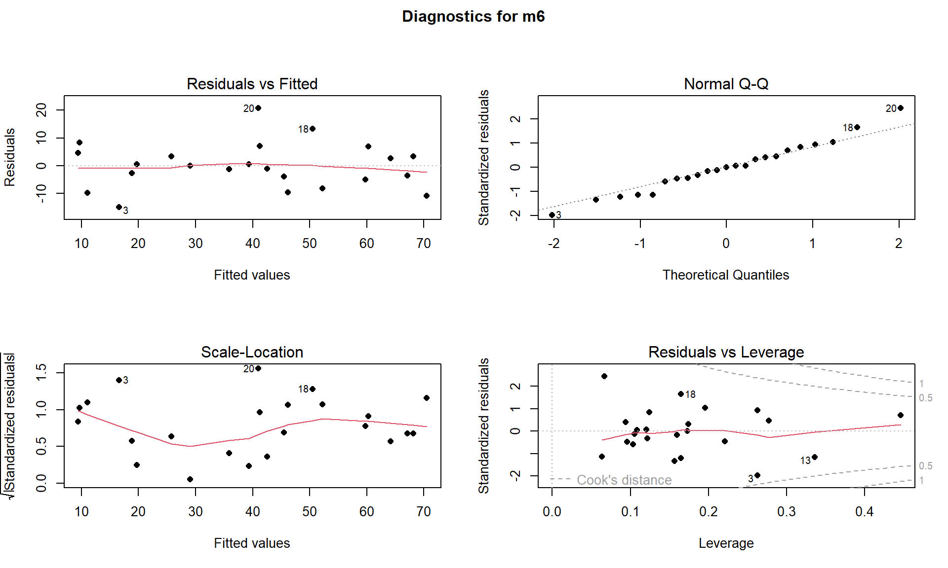

Figure 8.9: Diagnostic plots for MLR for Snow Depth based on Elevation, Min Temp and Max Temp with two observations removed (\(n = 23\)).

This worry-some observation is located in the 22^nd row of the original data set:

snotel_s %>% slice(22)

## # A tibble: 1 × 6
##      ID Station          Snow.Depth Max.Temp Min.Temp Elevation
##   <dbl> <fct>                 <dbl>    <dbl>    <dbl>     <dbl>
## 1    36 Bloody [Redact.]       27.2       39       26      7550

With the removal of both the “Northeast Entrance” and “Bloody \(\require{color}\colorbox{black}{Redact.}\)” sites, there are \(n = 23\) observations remaining. This model (m6) seems to contain residual diagnostics (Figure 8.9) that are finally generally reasonable.

m6 <- lm(Snow.Depth ~ Elevation + Min.Temp + Max.Temp, data = snotel_s %>% slice(-c(9,22)))
summary(m6)
par(mfrow = c(2,2), oma = c(0,0,2,0))
plot(m6, pch = 16, sub.caption = "")
title(main="Diagnostics for m6", outer=TRUE)

It is hard to suggest that there any curvature issues and the slight variation in the Scale-Location plot is mostly due to few observations with fitted values around 30 happening to be well approximated by the model. The normality assumption is generally reasonable and no points seem to be overly influential on this model (finally!).

The term-plots (Figure 8.10) show that the temperature slopes are both positive although in this model Max.Temp seems to be more “important” than Min.Temp. We have ruled out individual influential points as the source of un-expected directions in slope coefficients and the more likely issue is multicollinearity – in a model that includes Elevation, the temperature effects may be positive, again acting with the Elevation term to generate the best possible predictions of the observed responses. Throughout this discussion, we have mainly focused on the slope coefficients and diagnostics. We have other tools in MLR to more quantitatively assess and compare different regression models that are considered in the next sections.

plot(allEffects(m6, residuals = T), main = "MLR model with n = 23")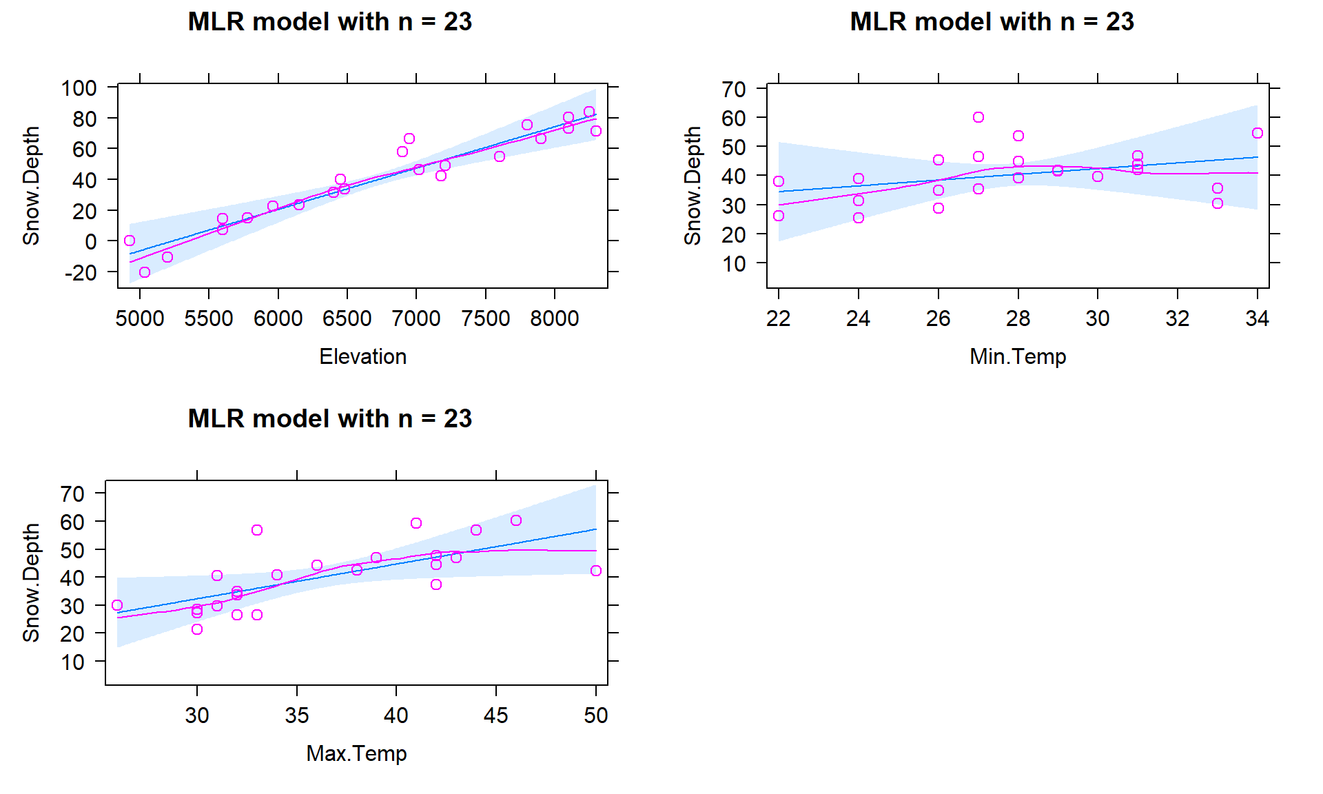

Figure 8.10: Term-plots for the MLR for Snow Depth based on Elevation, Min Temp and Max Temp with two observations removed.

As a final assessment of this model, we can consider simulating a set of \(n = 23\) responses from this model and then comparing that data set to the one we just analyzed. This does not change the predictor variables, but creates two new versions of the response called SimulatedSnow and SimulatedSnow2 in the following code chunk which are plotted in Figure 8.11. In exploring two realizations of simulated responses from the model, the results look fairly similar to the original data set. This model appeared to have reasonable assumptions and the match between simulated responses and the original ones reinforces those previous assessments. When the match is not so close, it can reinforce or create concern about the way that the assumptions have been assessed using other tools.

set.seed(307)
snotel_final <- snotel_s %>% slice(-c(9,22))
snotel_final <- snotel_final %>% 
  #Creates first and second set of simulated responses
  mutate(SimulatedSnow = simulate(m6)[[1]],
         SimulatedSnow2 = simulate(m6)[[1]]
         ) 

r1 <- snotel_final %>% ggplot(aes(x = Elevation, y = Snow.Depth)) + 
  geom_point() + 
  theme_bw() + 
  labs(title = "Real Responses")
r2 <- snotel_final %>% ggplot(aes(x = Max.Temp, y = Snow.Depth)) + 
  geom_point() + 
  theme_bw() + 
  labs(title = "Real Responses")
r3 <- snotel_final %>% ggplot(aes(x = Min.Temp, y = Snow.Depth)) + 
  geom_point() + 
  theme_bw() + 
  labs(title = "Real Responses")

s1 <- snotel_final %>% ggplot(aes(x = Elevation, y = SimulatedSnow)) + 
  geom_point(col = "forestgreen") + 
  theme_bw() + 
  labs(title = "First Simulated Responses")

s2 <- snotel_final %>% ggplot(aes(x = Max.Temp, y = SimulatedSnow)) + 
  geom_point(col = "forestgreen") + 
  theme_bw() + 
  labs(title = "First Simulated Responses")
s3 <- snotel_final %>% ggplot(aes(x = Min.Temp, y = SimulatedSnow)) + 
  geom_point(col = "forestgreen") + 
  theme_bw() + 
  labs(title = "First Simulated Responses")

s12 <- snotel_final %>% ggplot(aes(x = Elevation, y = SimulatedSnow2)) + 
  geom_point(col = "skyblue") + 
  theme_bw() + 
  labs(title = "Second Simulated Responses")
s22 <- snotel_final %>% ggplot(aes(x = Max.Temp, y = SimulatedSnow2)) + 
  geom_point(col = "skyblue") + 
  theme_bw() + 
  labs(title = "Second Simulated Responses")
s32 <- snotel_final %>% ggplot(aes(x = Min.Temp, y = SimulatedSnow2)) + 
  geom_point(col = "skyblue") + 
  theme_bw() + 
  labs(title = "Second Simulated Responses")

grid.arrange(r1, r2, r3, s1, s2, s3, s12, s22, s32, ncol = 3)

Figure 8.11: Plot of the original responses versus the three predictors (\(n\) = 23 data set) in the top row and two sets of simulated responses versus the predictors in the bottom two rows.