8.1: Going from SLR to MLR

In many situations, especially in observational studies, it is unlikely that the system is simple enough to be characterized by a single predictor variable. In experiments, if we randomly assign levels of a predictor variable we can assume that the impacts of other variables cancel out as a direct result of the random assignment. But it is possible even in these experimental situations that we can “improve” our model for the response variable by adding additional predictor variables that explain additional variation in the responses, reducing the amount of unexplained variation. This can allow more precise inferences to be generated from the model. As mentioned previously, it might be useful to know the sex or weight of the subjects in the Beers vs BAC study to account for more of the variation in the responses – this idea motivates our final topic: multiple linear regression (MLR) models. In observational studies, we can think of a suite of characteristics of observations that might be related to a response variable. For example, consider a study of yearly salaries and variables that might explain the amount people get paid. We might be most interested in seeing how incomes change based on age, but it would be hard to ignore potential differences based on sex and education level. Trying to explain incomes would likely require more than one predictor variable and we wouldn’t be able to explain all the variability in the responses just based on gender and education level, but a model using those variables might still provide some useful information about each component and about age impacts on income after we adjust (control) for sex and education. The extension to MLR allows us to incorporate multiple predictors into a regression model. Geometrically, this is a way of relating many different dimensions (number of \(x\text{'s}\)) to what happened in a single response variable (one dimension).

We start with the same model as in SLR except now we allow \(K\) different \(x\text{'s}\):

\[y_i = \beta_0 + \beta_1x_{1i} + \beta_2x_{2i}+ \ldots + \beta_Kx_{Ki} + \varepsilon_i\]

Note that if \(K = 1\), we are back to SLR. In the MLR model, there are \(K\) predictors and we still have a \(y\)-intercept. The MLR model carries the same assumptions as an SLR model with a couple of slight tweaks specific to MLR (see Section 8.2 for the details on the changes to the validity conditions).

We are able to use the least squares criterion for estimating the regression coefficients in MLR, but the mathematics are beyond the scope of this course. The lm function takes care of finding the least squares coefficients using a very sophisticated algorithm¹³². The estimated regression equation it returns is:

\[\widehat{y}_i = b_0 + b_1x_{1i} +b_2x_{2i}+\ldots+b_Kx_{Ki}\]

where each \(b_k\) estimates its corresponding parameter \(\beta_k\).

An example of snow depths at some high elevation locations in Montana on a day in April provides a nice motivation for these methods. A random sample of \(n = 25\) Montana locations (from the population of \(N = 85\) at the time) were obtained from the Natural Resources Conversation Service’s website (www.wcc.nrcs.usda.gov/snotel/Montana/montana.html) a few years ago. Information on the snow depth (Snow.Depth) in inches, daily Minimum and Maximum Temperatures (Min.Temp and Max.Temp) in \(^\circ F\) and elevation of the site (Elevation) in feet. A snow science researcher (or spring back-country skier) might be interested in understanding Snow depth as a function of Minimum Temperature, Maximum Temperature, and Elevation. One might assume that colder and higher places will have more snow, but using just one of the predictor variables might leave out some important predictive information. The following code loads the data set and makes the scatterplot matrix (Figure 8.1) to allow some preliminary assessment of the pairwise relationships.

snotel_s <- read_csv("http://www.math.montana.edu/courses/s217/documents/snotel_s.csv")

library(GGally)
# Reorder columns slightly and only plot quantitative variables using "columns = ..."
snotel_s %>% ggpairs(columns = c(4:6,3)) + 
  theme_bw()

Figure 8.1: Scatterplot matrix of data from a sample of SNOTEL sites in April on four variables.

It appears that there are many strong linear relationships between the variables, with Elevation and Snow Depth having the largest magnitude, r = 0.80. Higher temperatures seem to be associated with less snow – not a big surprise so far! There might be an outlier at an elevation of 7400 feet and a snow depth below 10 inches that we should explore further.

A new issue arises in attempting to build MLR models called multicollinearity. Again, it is a not surprise that temperature and elevation are correlated but that creates a problem if we try to put them both into a model to explain snow depth. Is it the elevation, temperature, or the combination of both that matters for getting and retaining more snow? Correlation between predictor variables is called multicollinearity and makes estimation and interpretation of MLR models more complicated than in SLR. Section 8.5 deals with this issue directly and discusses methods for detecting its presence. For now, remember that in MLR this issue sometimes makes it difficult to disentangle the impacts of different predictor variables on the response when the predictors share information – when they are correlated.

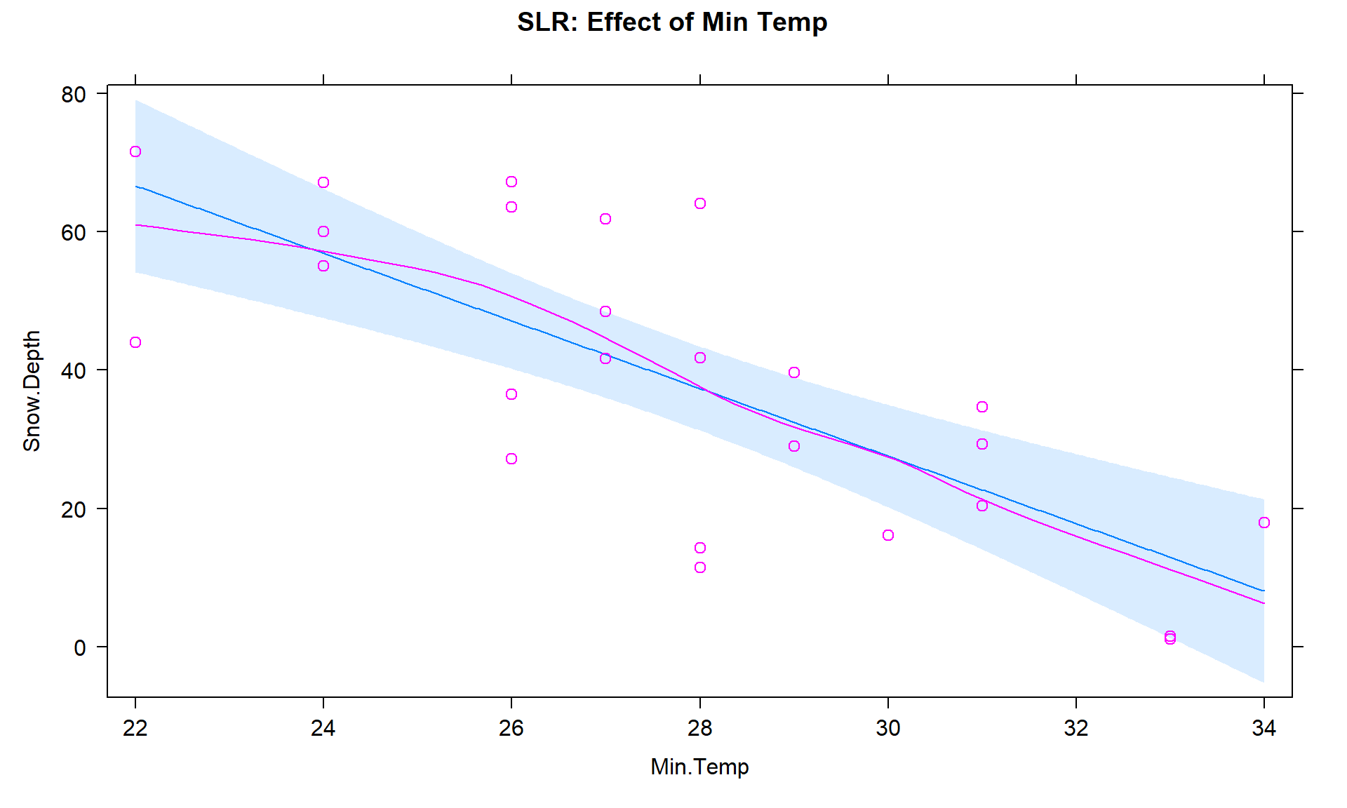
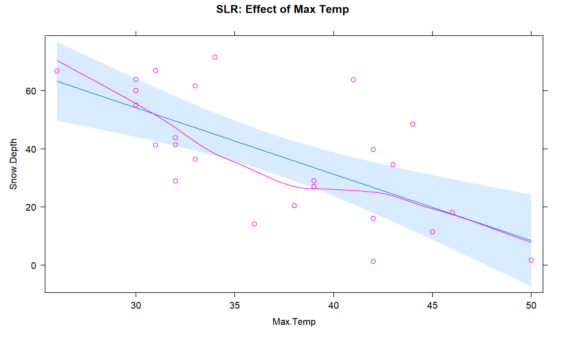
To get familiar with this example, we can start with fitting some potential SLR models and plotting the estimated models. Figure 8.2 contains the result for the SLR using Elevation and results for two temperature based models are in Figures 8.3 and 8.4. Snow Depth is selected as the obvious response variable both due to skier interest and potential scientific causation (snow can’t change elevation but elevation could be the driver of snow deposition and retention).

Figure 8.2: Plot of the estimated SLR model for Snow Depth with Elevation as the predictor along with observations and smoothing line generated by the residuals = T option being specified.

Based on the model summaries provided below, the three estimated SLR models are:

\[\begin{array}{rl} \widehat{\text{SnowDepth}}_i & = -72.006 + 0.0163\cdot\text{Elevation}_i, \\ \widehat{\text{SnowDepth}}_i & = 174.096 - 4.884\cdot\text{MinTemp}_i,\text{ and} \\ \widehat{\text{SnowDepth}}_i & = 122.672 - 2.284\cdot\text{MaxTemp}_i. \end{array}\]

The term-plots of the estimated models reinforce our expected results, showing a positive change in Snow Depth for higher Elevations and negative impacts for increasing temperatures on Snow Depth. These plots are made across the observed range¹³³ of the predictor variable and help us to get a sense of the total impacts of predictors. For example, for elevation in Figure 8.2, the smallest observed value was 4925 feet and the largest was 8300 feet. The regression line goes from estimating a mean snow depth of 8 inches to 63 inches. That gives you some practical idea of the size of the estimated Snow Depth change for the changes in Elevation observed in the data. Putting this together, we can say that there was around a 55 inch change in predicted snow depths for a close to 3400 foot increase in elevation. This helps make the slope coefficient of 0.0163 in the model more easily understood.

Remember that in SLR, the range of \(x\) matters just as much as the units of \(x\) in determining the practical importance and size of the slope coefficient. A value of 0.0163 looks small but is actually at the heart of a pretty interesting model for predicting snow depth. A one foot change of elevation is “tiny” here relative to changes in the response so the slope coefficient can be small and still amount to big changes in the predicted response across the range of values of \(x\). If the Elevation had been recorded in thousands of feet, then the slope would have been estimated to be \(0.0163*1000 = 16.3\) inches change in mean Snow Depth for a 1000 foot increase in elevation.

The plots of the two estimated temperature models in Figures 8.3 and 8.4 suggest a similar change in the responses over the range of observed temperatures. Those predictors range from 22\(^\circ F\) to 34\(^\circ F\) (minimum temperature) and from 26\(^\circ F\) to 50\(^\circ F\) (maximum temperature). This tells us a 1\(^\circ F\) increase in either temperature is a greater proportion of the observed range of each predictor than a 1 unit (foot) increase in elevation, so the two temperature variables will generate larger apparent magnitudes of slope coefficients. But having large slope coefficients is no guarantee of a good model – in fact, the elevation model has the highest R² value of these three models even though its slope coefficient looks tiny compared to the other models.

Figure 8.3: Plot of the estimated SLR model using Min Temp as predictor.

Figure 8.4: Plot of the estimated SLR model using Max Temp as predictor.

m1 <- lm(Snow.Depth ~ Elevation, data = snotel_s)
m2 <- lm(Snow.Depth ~ Min.Temp, data = snotel_s)
m3 <- lm(Snow.Depth ~ Max.Temp, data = snotel_s)
library(effects)
plot(allEffects(m1, residuals = T), main = "SLR: Effect of Elevation")
plot(allEffects(m2, residuals = T), main = "SLR: Effect of Min Temp")
plot(allEffects(m3, residuals = T), main = "SLR: Effect of Max Temp")

summary(m1)

## 
## Call:
## lm(formula = Snow.Depth ~ Elevation, data = snotel_s)
## 
## Residuals:
##     Min      1Q  Median      3Q     Max 
## -36.416  -5.135  -1.767   7.645  23.508 
## 
## Coefficients:
##               Estimate Std. Error t value Pr(>|t|)
## (Intercept) -72.005873  17.712927  -4.065 0.000478
## Elevation     0.016275   0.002579   6.311 1.93e-06
## 
## Residual standard error: 13.27 on 23 degrees of freedom
## Multiple R-squared:  0.634,  Adjusted R-squared:  0.618 
## F-statistic: 39.83 on 1 and 23 DF,  p-value: 1.933e-06

summary(m2)

## 
## Call:
## lm(formula = Snow.Depth ~ Min.Temp, data = snotel_s)
## 
## Residuals:
##     Min      1Q  Median      3Q     Max 
## -26.156 -11.238   2.810   9.846  26.444 
## 
## Coefficients:
##             Estimate Std. Error t value Pr(>|t|)
## (Intercept) 174.0963    25.5628   6.811 6.04e-07
## Min.Temp     -4.8836     0.9148  -5.339 2.02e-05
## 
## Residual standard error: 14.65 on 23 degrees of freedom
## Multiple R-squared:  0.5534, Adjusted R-squared:  0.534 
## F-statistic:  28.5 on 1 and 23 DF,  p-value: 2.022e-05

summary(m3)

## 
## Call:
## lm(formula = Snow.Depth ~ Max.Temp, data = snotel_s)
## 
## Residuals:
##     Min      1Q  Median      3Q     Max 
## -26.447 -10.367  -4.394  10.042  34.774 
## 
## Coefficients:
##             Estimate Std. Error t value Pr(>|t|)
## (Intercept) 122.6723    19.6380   6.247 2.25e-06
## Max.Temp     -2.2840     0.5257  -4.345 0.000238
## 
## Residual standard error: 16.25 on 23 degrees of freedom
## Multiple R-squared:  0.4508, Adjusted R-squared:  0.4269 
## F-statistic: 18.88 on 1 and 23 DF,  p-value: 0.0002385

Since all three variables look like they are potentially useful in predicting snow depth, we want to consider if an MLR model might explain more of the variability in Snow Depth. To fit an MLR model, we use the same general format as in previous topics but with adding “+” between any additional predictors¹³⁴ we want to add to the model, y ~ x1 + x2 + ... + xk:

m4 <- lm(Snow.Depth ~ Elevation + Min.Temp + Max.Temp, data = snotel_s)
summary(m4)

## 
## Call:
## lm(formula = Snow.Depth ~ Elevation + Min.Temp + Max.Temp, data = snotel_s)
## 
## Residuals:
##     Min      1Q  Median      3Q     Max 
## -29.508  -7.679  -3.139   9.627  26.394 
## 
## Coefficients:
##               Estimate Std. Error t value Pr(>|t|)
## (Intercept) -10.506529  99.616286  -0.105   0.9170
## Elevation     0.012332   0.006536   1.887   0.0731
## Min.Temp     -0.504970   2.042614  -0.247   0.8071
## Max.Temp     -0.561892   0.673219  -0.835   0.4133
## 
## Residual standard error: 13.6 on 21 degrees of freedom
## Multiple R-squared:  0.6485, Adjusted R-squared:  0.5983 
## F-statistic: 12.91 on 3 and 21 DF,  p-value: 5.328e-05

plot(allEffects(m4, residuals = T), main = "MLR model with Elev, Min, & Max Temps")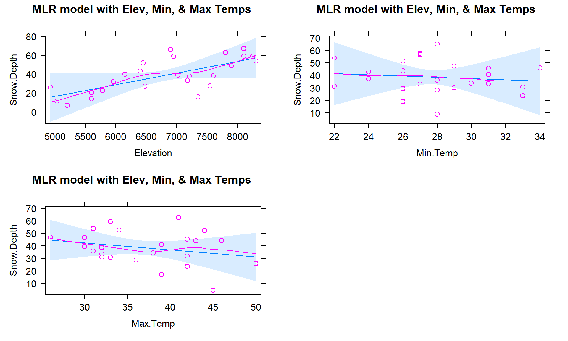

Figure 8.5: Term-plots for the MLR for Snow Depth based on Elevation, Min Temp and Max Temp. Compare this plot that comes from one MLR model to Figures 8.2, 8.3, and 8.4 for comparable SLR models. Note the points in these panels are the partial residuals that are generated after controlling for the other two of the three variables as explained below.

Based on the output, the estimated MLR model is

\[\widehat{\text{SnowDepth}}_i = -10.51 + 0.0123\cdot\text{Elevation}_i -0.505\cdot\text{MinTemp}_i - 0.562\cdot\text{MaxTemp}_i\]

The direction of the estimated slope coefficients were similar but they all changed in magnitude as compared to the respective SLRs, as seen in the estimated term-plots from the MLR model in Figure 8.5.

There are two ways to think about the changes from individual SLR slope coefficients to the similar MLR results here.

1. Each term in the MLR is the result for estimating each slope after controlling for the other two variables (and we will always use this sort of interpretation any time we interpret MLR effects). For the Elevation slope, we would say that the slope coefficient is “corrected for” or “adjusted for” the variability that is explained by the temperature variables in the model.
2. Because of multicollinearity in the predictors, the variables might share information that is useful for explaining the variability in the response variable, so the slope coefficients of each predictor get perturbed because the model cannot separate their effects on the response. This issue disappears when the predictors are uncorrelated or even just minimally correlated.

There are some ramifications of multicollinearity in MLR:

1. Adding variables to a model might lead to almost no improvement in the overall variability explained by the model.
2. Adding variables to a model can cause slope coefficients to change signs as well as magnitudes.
3. Adding variables to a model can lead to inflated standard errors for some or all of the coefficients (this is less obvious but is related to the shared information in predictors making it less clear what slope coefficient to use for each variable, so more uncertainty in their estimation).
4. In extreme cases of multicollinearity, it may even be impossible to obtain some or any coefficient estimates.

These seem like pretty serious issues and they are but there are many, many situations where we proceed with MLR even in the presence of potentially correlated predictors. It is likely that you have heard or read about inferences from models that are dealing with this issue – for example, medical studies often report the increased risk of death from some behavior or trait after controlling for gender, age, health status, etc. In many research articles, it is becoming common practice to report the slope for a variable that is of most interest with it in the model alone (SLR) and in models after adjusting for the other variables that are expected to matter. The “adjusted for other variables” results are built with MLR or related multiple-predictor models like MLR.