7.5: Transformations part I - Linearizing relationships

When the influential point, linearity, constant variance and/or normality assumptions are clearly violated, we cannot trust any of the inferences generated by the regression model. The violations occur on gradients from minor to really major problems. As we have seen from the examples in the previous chapters, it has been hard to find data sets that were free of all issues. Furthermore, it may seem hopeless to be able to make successful inferences in some of these situations with the previous tools. There are three potential solutions to violations of the validity conditions:

1. Consider removing an offending point or two and see if this improves the results, presenting results both with and without those points to describe their impact¹²⁵,
2. Try to transform the response, explanatory, or both variables and see if you can force the data set to meet our SLR assumptions after transformation (the focus of this and the next section), or
3. Consider more advanced statistical models that can account for these issues (the focus of subsequent statistics courses, if you continue on further).

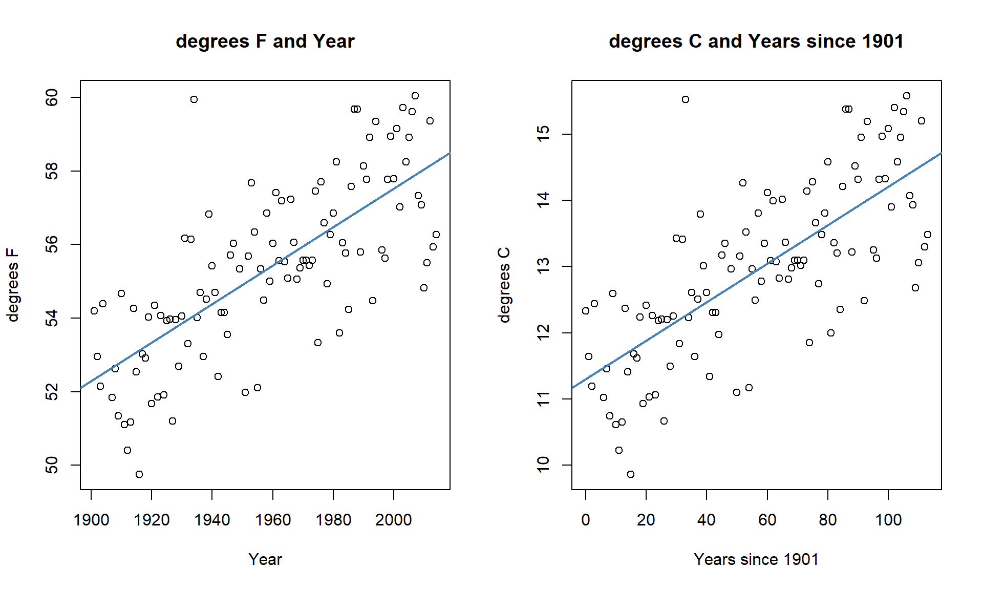
Transformations involve applying a function to one or both variables. After applying this transformation, one hopes to have alleviated whatever issues encouraged its consideration. Linear transformation functions, of the form \(z_{\text{new}} = a*x+b\), will never help us to fix assumptions in regression situations; linear transformations change the scaling of the variables but not their shape or the relationship between two variables. For example, in the Bozeman Temperature data example, we subtracted 1901 from the Year variable to have Year2 start at 0 and go up to 113. We could also apply a linear transformation to change Temperature from being measured in \(^\circ F\) to \(^\circ C\) using \(^\circ C = [^\circ F - 32] *(5/9)\). The scatterplots on both the original and transformed scales are provided in Figure 7.11. All the coefficients in the regression model and the labels on the axes change, but the “picture” is still the same. Additionally, all the inferences remain the same – p-values are unchanged by linear transformations. So linear transformations can be “fun” but really are only useful if they make the coefficients easier to interpret. Here if you like temperature changes in \(^\circ C\) for a 1 year increase, the slope coefficient is 0.029 and if you like the original change in \(^\circ F\) for a 1 year increase, the slope coefficient is 0.052. More useful than this is the switch into units of 100 years (so each year increase would just be 0.1 instead of 1), so that the slope is the temperature change over 100 years.

Figure 7.11: Scatterplots of Temperature (\(^\circ F\)) versus Year (left) and Temperature (\(^\circ C\)) vs Years since 1901 (right).

bozemantemps <- bozemantemps %>% mutate(meanmaxC = (meanmax - 32)*(5/9))
temp3 <- lm(meanmaxC ~ Year2, data = bozemantemps)
summary(temp1)

## 
## Call:
## lm(formula = meanmax ~ Year, data = bozemantemps)
## 
## Residuals:
##     Min      1Q  Median      3Q     Max 
## -3.3779 -0.9300  0.1078  1.1960  5.8698 
## 
## Coefficients:
##              Estimate Std. Error t value Pr(>|t|)
## (Intercept) -47.35123    9.32184   -5.08 1.61e-06
## Year          0.05244    0.00476   11.02  < 2e-16
## 
## Residual standard error: 1.624 on 107 degrees of freedom
## Multiple R-squared:  0.5315, Adjusted R-squared:  0.5271 
## F-statistic: 121.4 on 1 and 107 DF,  p-value: < 2.2e-16

summary(temp3)

## 
## Call:
## lm(formula = meanmaxC ~ Year2, data = bozemantemps)
## 
## Residuals:
##     Min      1Q  Median      3Q     Max 
## -1.8766 -0.5167  0.0599  0.6644  3.2610 
## 
## Coefficients:
##              Estimate Std. Error t value Pr(>|t|)
## (Intercept) 11.300703   0.174349   64.82   <2e-16
## Year2        0.029135   0.002644   11.02   <2e-16
## 
## Residual standard error: 0.9022 on 107 degrees of freedom
## Multiple R-squared:  0.5315, Adjusted R-squared:  0.5271 
## F-statistic: 121.4 on 1 and 107 DF,  p-value: < 2.2e-16

Nonlinear transformation functions are where we apply something more complicated than this shift and scaling, something like \(y_{\text{new}} = f(y)\), where \(f(\cdot)\) could be a log or power of the original variable \(y\). When we apply these sorts of transformations, interesting things can happen to our linear models and their problems. Some examples of transformations that are at least occasionally used for transforming the response variable are provided in Table 7.1, ranging from taking \(y\) to different powers from \(y^{-2}\) to \(y^2\). Typical transformations used in statistical modeling exist along a gradient of powers of the response variable, defined as \(y^{\lambda}\) with \(\boldsymbol{\lambda}\) being the power of the transformation of the response variable and \(\lambda = 0\) implying a log-transformation. Except for \(\lambda = 1\), the transformations are all nonlinear functions of \(y\).

Table 7.1: Ladder of powers of transformations that are often used in statistical modeling.

Power	Formula	Usage
2	\(y^2\)	seldom used
1	\(y^1=y\)	no change
\(1/2\)	\(y^{0.5}=\sqrt{y}\)	counts and area responses
0	\(\log(y)\) natural log of \(y\)	counts, normality, curves, non-constant variance
\(-1/2\)	\(y^{-0.5}=1/\sqrt{y}\)	uncommon
\(-1\)	\(y^{-1}=1/y\)	for ratios
\(-2\)	\(y^{-2}=1/y^2\)	seldom used

There are even more transformations possible, for example \(y^{0.33}\) is sometimes useful for variables involved in measuring the volume of something. And we can also consider applying any of these transformations to the explanatory variable, and consider using them on both the response and explanatory variables at the same time. The most common application of these ideas is to transform the response variable using the log-transformation, at least as a starting point. In fact, the log-transformation is so commonly used (or maybe overused), that we will just focus on its use. It is so commonplace in some fields that some researchers log-transform their data prior to even plotting it. In other situations, such as when measuring acidity (pH), noise (decibels), or earthquake size (Richter scale), the measurements are already on logarithmic scales.

Actually, we have already analyzed data that benefited from a log-transformation – the log-area burned vs. summer temperature data for Montana. Figure 7.12 compares the relationship between these variables on the original hectares scale and the log-hectares scale.

p <- mtfires %>% ggplot(mapping = aes(x = Temperature, y = hectares)) +
  geom_point() +
  labs(title = "(a)", y = "Hectares") +
  theme_bw()
            
plog <- mtfires %>% ggplot(mapping = aes(x = Temperature, y = loghectares)) +
  geom_point() +
  labs(title = "(b)", y = "log-Hectares") +
  theme_bw()

grid.arrange(p, plog, ncol = 2)

Figure 7.12: Scatterplots of Hectares (a) and log-Hectares (b) vs Temperature.

Figure 7.12(a) displays a relationship that would be hard fit using SLR – it has a curve and the variance is increasing with increasing temperatures. With a log-transformation of Hectares, the relationship appears to be relatively linear and have constant variance (in (b)). We considered regression models for this situation previously. This shows at least one situation where a log-transformation of a response variable can linearize a relationship and reduce non-constant variance.

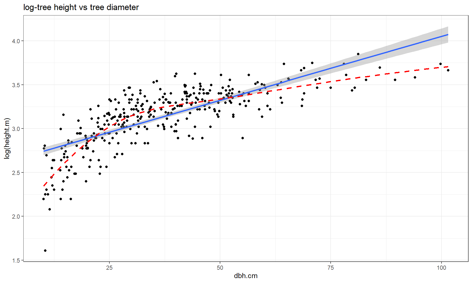
This transformation does not always work to “fix” curvilinear relationships, in fact in some situations it can make the relationship more nonlinear. For example, reconsider the relationship between tree diameter and tree height, which contained some curvature that we could not account for in an SLR. Figure 7.13 shows the original version of the variables and Figure 7.14 shows the same information with the response variable (height) log-transformed.

library(spuRs)
data(ufc)
ufc <- as_tibble(ufc)
ufc %>% slice(-168) %>% ggplot(mapping = aes(x = dbh.cm, y = height.m)) +
  geom_point() +
  geom_smooth(method = "lm") +
  geom_smooth(col = "red", lwd = 1, se = F, lty = 2) +
  theme_bw() +
  labs(title = "Tree height vs tree diameter")

ufc %>% slice(-168) %>% ggplot(mapping = aes(x = dbh.cm, y = log(height.m))) +
  geom_point() +
  geom_smooth(method = "lm") +
  geom_smooth(col = "red", lwd = 1, se = F, lty = 2) +
  theme_bw() +
  labs(title = "log-tree height vs tree diameter")

Figure 7.13: Scatterplot of tree height versus tree diameter.

Figure 7.14 with the log-transformed height response seems to show a more nonlinear relationship and may even have more issues with non-constant variance. This example shows that log-transforming the response variable cannot fix all problems, even though I’ve seen some researchers assume it can. It is OK to try a transformation but remember to always plot the results to make sure it actually helped and did not make the situation worse.

Figure 7.14: Scatterplot of log(tree height) versus tree diameter.

All is not lost in this situation, we can consider two other potential uses of the log-transformation and see if they can “fix” the relationship up a bit. One option is to apply the transformation to the explanatory variable (y ~ log(x)), displayed in Figure 7.15. If the distribution of the explanatory variable is right skewed (see the boxplot on the \(x\)-axis), then consider log-transforming the explanatory variable. This will often reduce the leverage of those most extreme observations which can be useful. In this situation, it also seems to have been quite successful at linearizing the relationship, leaving some minor non-constant variance, but providing a big improvement from the relationship on the original scale.

Figure 7.15: Scatterplot of tree height versus log(tree diameter).

The other option, especially when everything else fails, is to apply the log-transformation to both the explanatory and response variables (log(y) ~ log(x)), as displayed in Figure 7.16. For this example, the transformation seems to be better than the first two options (none and only \(\log(y)\)), but demonstrates some decreasing variability with larger \(x\) and \(y\) values. It has also created a new and different curve in the relationship (see the smoothing (dashed) line start below the SLR line, then go above it, and the finish below it). In the end, we might prefer to fit an SLR model to the tree height vs log(diameter) versions of the variables (Figure 7.15).

ufc %>% slice(-168) %>% ggplot(mapping = aes(x = log(dbh.cm), y = log(height.m))) +
  geom_point() +
  geom_smooth(method = "lm") +
  geom_smooth(col = "red", lwd = 1, se = F, lty = 2) +
  theme_bw() +
  labs(title = "log-tree height vs log-tree diameter")

Figure 7.16: Scatterplot of log(tree height) versus log(tree diameter).

Economists also like to use \(\log(y) \sim \log(x)\) transformations. The log-log transformation tends to linearize certain relationships and has specific interpretations in terms of Economics theory. The log-log transformation shows up in many different disciplines as a way of obtaining a linear relationship on the log-log scale, but different fields discuss it differently. The following example shows a situation where transformations of both \(x\) and \(y\) are required and this double transformation seems to be quite successful in what looks like an initially hopeless situation for our linear modeling approach.

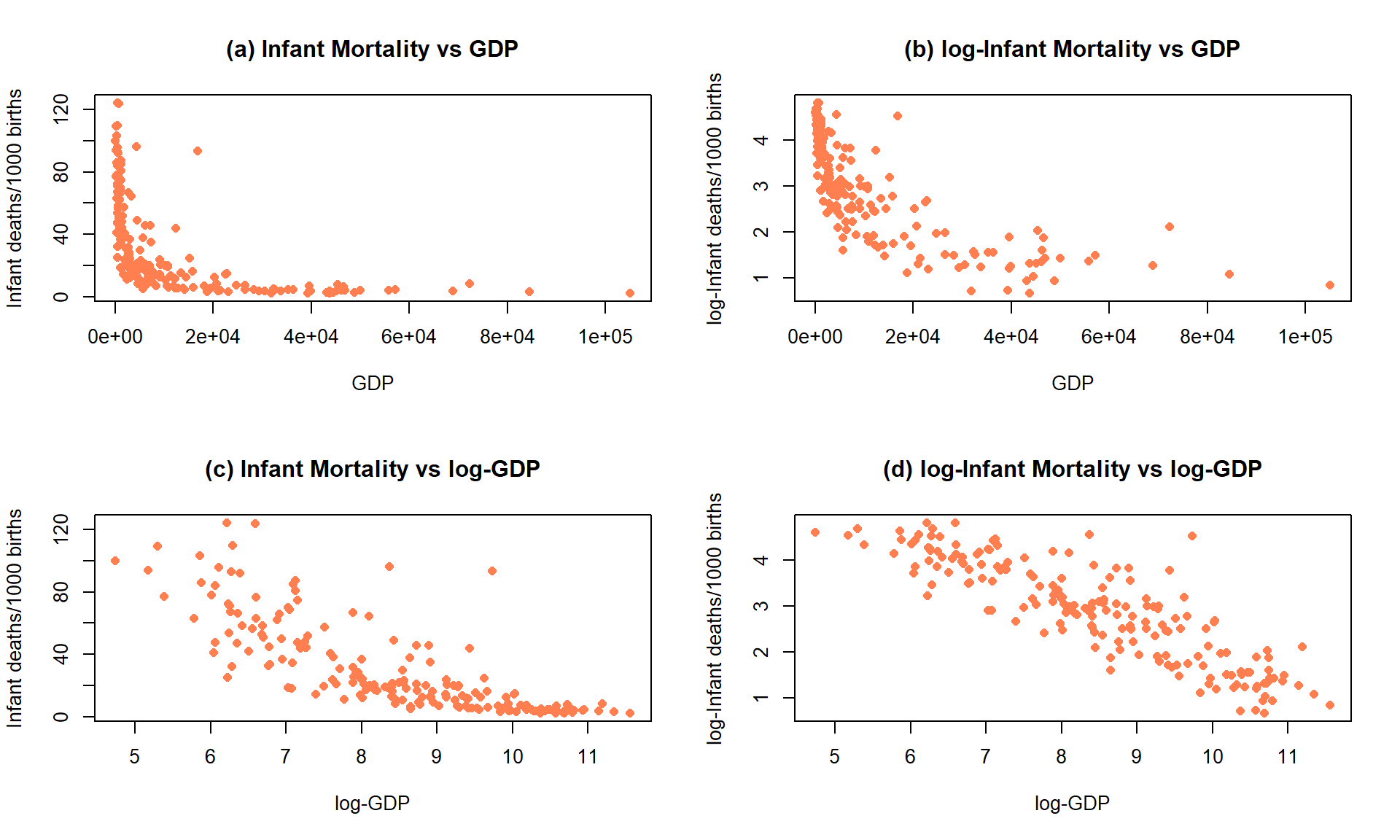
Data were collected in 1988 on the rates of infant mortality (infant deaths per 1,000 live births) and gross domestic product (GDP) per capita (in 1998 US dollars) from \(n = 207\) countries. These data are available from the carData package (Fox, Weisberg, and Price (2022b), Fox (2003)) in a data set called UN. The four panels in Figure 7.17 show the original relationship and the impacts of log-transforming one or both variables. The only scatterplot that could potentially be modeled using SLR is the lower right panel (d) that shows the relationship between log(infant mortality) and log(GDP). In the next section, we will fit models to some of these relationships and use our diagnostic plots to help us assess “success” of the transformations.

Figure 7.17: Scatterplots of Infant Mortality vs GDP under four different combinations of log-transformations.

Almost all nonlinear transformations assume that the variables are strictly greater than 0. For example, consider what happens when we apply the log function to 0 or a negative value in R:

log(-1)

## [1] NaN

log(0)

## [1] -Inf

So be careful to think about the domain of the transformation function before using transformations. For example, when using the log-transformation make sure that the data values are non-zero and positive or you will get some surprises when you go to fit your regression model to a data set with NaNs (not a number) and/or \(-\infty\text{'s}\) in it. When using fractional powers (square-roots or similar), just having non-negative values are required and so 0 is acceptable.

Sometimes the log-transformations will not be entirely successful. If the relationship is monotonic (strictly positive or strictly negative but not both), then possibly another stop on the ladder of transformations in Table 7.1 might work. If the relationship is not monotonic, then it may be better to consider a more complex regression model that can accommodate the shape in the relationship or to bin the predictor, response, or both into categories so you can use ANOVA or Chi-square methods and avoid at least the linearity assumption.

Finally, remember that log in statistics and especially in R means the natural log (ln or log base e as you might see it elsewhere). In these situations, applying the log10 function (which provides log base 10) to the variables would lead to very similar results, but readers may assume you used ln if you don’t state that you used \(log_{10}\). The main thing to remember to do is to be clear when communicating the version you are using. As an example, I was working with researchers on a study (Dieser, Greenwood, and Foreman 2010) related to impacts of environmental stresses on bacterial survival. The response variable was log-transformed counts and involved smoothed regression lines fit on this scale. I was using natural logs to fit the models and then shared the fitted values from the models and my collaborators back-transformed the results assuming that I had used \(log_{10}\). We quickly resolved our differences once we discovered them but this serves as a reminder at how important communication is in group projects – we both said we were working with log-transformations and didn’t know that we defaulted to different bases.

Generally, in statistics, it’s safe to assume that everything is log base e unless otherwise specified.