7.6: Transformations part II - Impacts on SLR interpretations - log(y), log(x), and both log(y) and log(x)

The previous attempts to linearize relationships imply a desire to be able to fit SLR models. The log-transformations, when successful, provide the potential to validly apply our SLR model. There are then two options for interpretations: you can either interpret the model on the transformed scale or you can translate the SLR model on the transformed scale back to the original scale of the variables. It ends up that log-transformations have special interpretations on the original scales depending on whether the log was applied to the response variable, the explanatory variable, or both.

Scenario 1: log(y) vs x model:

First consider the \(\log(y) \sim x\) situations where the estimated model is of the form \(\widehat{\log(y)} = b_0 + b_1x\). When only the response is log-transformed, some people call this a semi-log model. But many researchers will use this model without any special considerations, as long as it provides a situation where the SLR assumptions are reasonably well-satisfied. To understand the properties and eventually the interpretation of transformed-variables models, we need to try to “reverse” our transformation. If we exponentiate¹²⁶ both sides of \(\log(y) = b_0 + b_1x\), we get:

Figure 7.18: Plot of the estimated SLR (a) and implied model for the median on the original Hectares scale (b) for the area burned vs temperature data.

• \(\exp(\log(y)) = \exp(b_0 + b_1x)\), which is
• \(y = \exp(b_0 + b_1x)\), which can be re-written as
• \(y = \exp(b_0)\exp(b_1x)\). This is based on the rules for exp() where \(\exp(a+b) = \exp(a)\exp(b)\).
• Now consider what happens if we increase \(x\) by 1 unit, going from \(x\) to \(x+1\), providing a new predicted \(y\) that we can call \(y^*\): \(y^* = \exp(b_0)\exp[b_1(x+1)]\):
• \(y^* = {\color{red}{\underline{\boldsymbol{\exp(b_0)\exp(b_1x)}}}}\exp(b_1)\). Now note that the underlined, bold component was the y-value for \(x\).
• \(y^* = {\color{red}{\boldsymbol{y}}}\exp(b_1)\). Found by replacing \(\color{red}{\mathbf{\exp(b_0)\exp(b_1x)}}\) with \(\color{red}{\mathbf{y}}\), the value for \(x\).

So the difference in fitted values between \(x\) and \(x+1\) is to multiply the result for \(x\) (that was predicting \(\color{red}{\mathbf{y}}\)) by \(\exp(b_1)\) to get to the predicted result for \(x+1\) (called \(y^*\)). We can then use this result to form our \(\mathit{\boldsymbol{\log(y)\sim x}}\) slope interpretation: for a 1 unit increase in \(x\), we observe a multiplicative change of \(\mathbf{exp(b_1)}\) in the response. When we compute a mean on logged variables that are symmetrically distributed (this should occur if our transformation was successful) and then exponentiate the results, the proper interpretation is that the changes are happening in the median of the original responses. This is the only time in the course that we will switch our inferences to medians instead of means, and we don’t do this because we want to, we do it because it is result of modeling on the \(\log(y)\) scale, if successful.

So there are a couple of ways to interpret these results in general:

1. log-scale interpretation of log(y) only model: for a 1 unit increase in \(x\), we estimate a \(b_1\) unit change in the mean of \(\log(y)\) or
2. original scale interpretation of log(y) only model: for a 1 unit increase in \(x\), we estimate a \(exp(b_1)\) times change in the median of \(y\).

When we are working with regression equations, slopes can either be positive or negative and our interpretations change based on this result to either result in growth (\(b_1>0\)) or decay (\(b_1<0\)) in the responses as the explanatory variable is increased. As an example, consider \(b_1 = 0.4\) and \(\exp(b_1) = \exp(0.4) = 1.492\). There are a couple of ways to interpret this on the original scale of the response variable \(y\):

For \(\mathbf{b_1>0}\):

1. For a 1 unit increase in \(x\), the median of \(y\) is estimated to change by 1.492 times.
2. We can convert this into a percentage increase by subtracting 1 from \(\exp(0.4)\), \(1.492-1.0 = 0.492\) and multiplying the result by 100, \(0.492*100 = 49.2\%\). This is interpreted as: For a 1 unit increase in \(x\), the median of \(y\) is estimated to increase by 49.2%.

exp(0.4)

## [1] 1.491825

For \(\mathbf{b_1<0}\), the change on the log-scale is negative and that implies on the original scale that the curve decays to 0. For example, consider \(b_1 = -0.3\) and \(\exp(-0.3) = 0.741\). Again, there are two versions of the interpretation possible:

1. For a 1 unit increase in \(x\), the median of \(y\) is estimated to change by 0.741 times.
2. For negative slope coefficients, the percentage decrease is calculated as \((1-\exp(b_1))*100\%\). For \(\exp(-0.3) = 0.741\), this is \((1-0.741)*100 = 25.9\%\). This is interpreted as: For a 1 unit increase in \(x\), the median of \(y\) is estimated to decrease by 25.9%.

We suspect that you will typically prefer the “times” interpretation over the “percentage” change one for both directions but it is important to be able think about the results in terms of % change of the medians to make the scale of change more understandable. Some examples will help us see how these ideas can be used in applications.

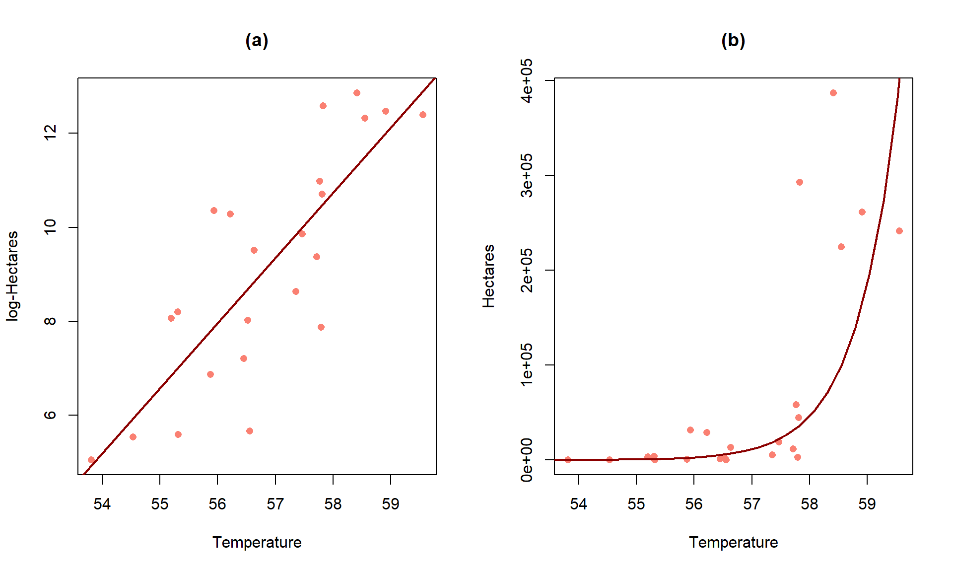
For the area burned data set, the estimated regression model is \(\log(\widehat{\text{hectares}}) = -69.8+1.39\cdot\text{ Temp}\). On the original scale, this implies that the model is \(\widehat{\text{hectares}} = \exp(-69.8)\exp(1.39\text{ Temp})\). Figure 7.18 provides the \(\log(y)\) scale version of the model and the model transformed to the original scale of measurement. On the log-hectares scale, the interpretation of the slope is: For a 1\(^\circ F\) increase in summer temperature, we estimate a 1.39 log-hectares/1\(^\circ F\) change, on average, in the log-area burned. On the original scale: A 1\(^\circ F\) increase in temperature is related to an estimated multiplicative change in the median number of hectares burned of \(\exp(1.39) = 4.01\) times higher areas. That seems like a big rate of growth but the curve does grow rapidly as shown in panel (b), especially for values over 58\(^\circ F\) where the area burned is starting to be really large. You can think of the multiplicative change here in the following way: the median number of hectares burned is 4 times higher at 58\(^\circ F\) than at 57\(^\circ F\) and the median area burned is 4 times larger at 59\(^\circ F\) than at 58\(^\circ F\)… This can also be interpreted on a % change scale: A 1\(^\circ F\) increase in temperature is related to an estimated \((4.01-1)*100 = 301\%\) increase in the median number of hectares burned.

Scenario 2: y vs log(x) model:

When only the explanatory variable is log-transformed, it has a different sort of impact on the regression model interpretation. Effectively we move the percentage change onto the \(x\)-scale and modify the first part of our slope interpretation when we consider the results on the original scale for \(x\). Once again, we will consider the mathematics underlying the changes in the model and then work on applying it to real situations. When the explanatory variable is logged, the estimated regression model is \(\color{red}{\boldsymbol{y = b_0+b_1\log(x)}}\). This models the relationship between \(y\) and \(x\) in terms of multiplicative changes in \(x\) having an effect on the average \(y\).

To develop an interpretation on the \(x\)-scale (not \(\log(x)\)), consider the impact of doubling \(x\). This change will take us from the point (\(x,\color{red}{\boldsymbol{y = b_0+b_1\log(x)}}\)) to the point \((2x,\boldsymbol{y^* = b_0+b_1\log(2x)})\). Now the impact of doubling \(x\) can be simplified using the rules for logs to be:

• \(\boldsymbol{y^* = b_0+b_1\log(2x)}\),
• \(\boldsymbol{y^*} = {\color{red}{\underline{\boldsymbol{b_0+b_1\log(x)}}}} + b_1\log(2)\). Based on the rules for logs: \(log(2x) = log(x)+log(2)\).
• \(y^* = {\color{red}{\boldsymbol{y}}}+b_1\log(2)\)
• So if we double \(x\), we change the mean of \(y\) by \(b_1\log(2)\).

As before, there are couple of ways to interpret these sorts of results,

1. log-scale interpretation of log(x) only model: for a 1 log-unit increase in \(x\), we estimate a \(b_1\) unit change in the mean of \(y\) or
2. original scale interpretation of log(x) only model: for a doubling of \(x\), we estimate a \(b_1\log(2)\) change in the mean of \(y\). Note that both interpretations are for the mean of the \(y\text{'s}\) since we haven’t changed the \(y\sim\) part of the model.

Figure 7.19: Plot of the observations and estimated SLR model (mortality ~ log(GDP)) (top) and implied model (bottom) for the infant mortality data.

While it is not a perfect model (no model is), let’s consider the model for infant mortality \(\sim\) log(GDP) in order to practice the interpretation using this type of model. This model was estimated to be \(\widehat{\text{infantmortality}} = 155.77-14.86\cdot\log(\text{GDP})\). The first (simplest) interpretation of the slope coefficient is: For a 1 log-dollar increase in GDP per capita, we estimate infant mortality to change, on average, by -14.86 deaths/1000 live births. The second interpretation is on the original GDP scale: For a doubling of GDP, we estimate infant mortality to change, on average, by \(-14.86\log(2) = -10.3\) deaths/1000 live births. Or, the mean infant mortality is reduced by 10.3 deaths per 1000 live births for each doubling of GDP. Both versions of the model are displayed in Figure 7.19 – one on the scale the SLR model was fit (panel a) and the other on the original \(x\)-scale (panel b) that matches these last interpretations.

ID1 <- lm(infantMortality ~ log(ppgdp), data = UN)
summary(ID1)

## 
## Call:
## lm(formula = infantMortality ~ log(ppgdp), data = UN)
## 
## Residuals:
##     Min      1Q  Median      3Q     Max 
## -38.239 -11.609  -2.829   8.122  82.183 
## 
## Coefficients:
##             Estimate Std. Error t value Pr(>|t|)
## (Intercept) 155.7698     7.2431   21.51   <2e-16
## log(ppgdp)  -14.8617     0.8468  -17.55   <2e-16
## 
## Residual standard error: 18.14 on 191 degrees of freedom
## Multiple R-squared:  0.6172, Adjusted R-squared:  0.6152 
## F-statistic:   308 on 1 and 191 DF,  p-value: < 2.2e-16

-14.86*log(2)

## [1] -10.30017

It appears that our model does not fit too well and that there might be some non-constant variance so we should check the diagnostic plots (available in Figure 7.20) before we trust any of those previous interpretations.

par(mfrow = c(2,2))
plot(ID1)

Figure 7.20: Diagnostics plots of the infant mortality model with log(GDP).

There appear to be issues with outliers and a long right tail violating the normality assumption as it suggests a clear right skewed residual distribution. There is curvature and non-constant variance in the results as well. There are no influential points, but we are far from happy with this model and will be revisiting this example with the responses also transformed. Remember that the log-transformation of the response can potentially fix non-constant variance, normality, and curvature issues.

Scenario 3: log(y) ~ log(x) model

A final model combines log-transformations of both \(x\) and \(y\), combining the interpretations used in the previous two situations. This model is called the log-log model and in some fields is also called the power law model. The power-law model is usually written as \(y = \beta_0x^{\beta_1}+\varepsilon\), where \(y\) is thought to be proportional to \(x\) raised to an estimated power of \(\beta_1\) (linear if \(\beta_1 = 1\) and quadratic if \(\beta_1 = 2\)). It is one of the models that has been used in Geomorphology to model the shape of glaciated valley elevation profiles (that classic U-shape that comes with glacier-eroded mountain valleys)¹²⁷. If you ignore the error term, it is possible to estimate the power-law model using our SLR approach. Consider the log-transformation of both sides of this equation starting with the power-law version:

• \(\log(y) = \log(\beta_0x^{\beta_1})\),
• \(\log(y) = \log(\beta_0) + \log(x^{\beta_1}).\) Based on the rules for logs: \(\log(ab) = \log(a) + \log(b)\).
• \(\log(y) = \log(\beta_0) + \beta_1\log(x).\) Based on the rules for logs: \(\log(x^b) = b\log(x)\).

Figure 7.21: Plot of the observations and estimated SLR model log(mortality) \(\sim\) log(GDP) (left) and implied model (right) for the infant mortality data.

So other than \(\log(\beta_0)\) in the model, this looks just like our regular SLR model with \(x\) and \(y\) both log-transformed. The slope coefficient for \(\log(x)\) is the power coefficient in the original power law model and determines whether the relationship between the original \(x\) and \(y\) in \(y = \beta_0x^{\beta_1}\) is linear \((y = \beta_0x^1)\) or quadratic \((y = \beta_0x^2)\) or even quartic \((y = \beta_0x^4)\) in some really heavily glacier carved U-shaped valleys. There are some issues with “ignoring the errors” in using SLR to estimate these models (M. C. Greenwood and Humphrey 2002) but it is still a pretty powerful result to be able to estimate the coefficients in \((y = \beta_0x^{\beta_1})\) using SLR.

We don’t typically use the previous ideas to interpret the typical log-log regression model, instead we combine our two previous interpretation techniques to generate our interpretation.

We need to work out the mathematics of doubling \(x\) and the changes in \(y\) starting with the \(\mathit{\boldsymbol{\log(y)\sim \log(x)}}\) model that we would get out of fitting the SLR with both variables log-transformed:

• \(\log(y) = b_0 + b_1\log(x)\),
• \(y = \exp(b_0 + b_1\log(x))\). Exponentiate both sides.
• \(y = \exp(b_0)\exp(b_1\log(x)) = \exp(b_0)x^{b_1}\). Rules for exponents and logs, simplifying.

Now we can consider the impacts of doubling \(x\) on \(y\), going from \((x,{\color{red}{\boldsymbol{y = \exp(b_0)x^{b_1}}}})\) to \((2x,y^*)\) with

• \(y^* = \exp(b_0)(2x)^{b_1}\),
• \(y^* = \exp(b_0)2^{b_1}x^{b_1} = 2^{b_1}{\color{red}{\boldsymbol{\exp(b_0)x^{b_1}}}} = 2^{b_1}{\color{red}{\boldsymbol{y}}}\)

So doubling \(x\) leads to a multiplicative change in the median of \(y\) of \(2^{b_1}\).

Let’s apply this idea to the GDP and infant mortality data where a \(\log(x) \sim \log(y)\) transformation actually made the resulting relationship look like it might be close to being reasonably modeled with an SLR. The regression line in Figure 7.21 actually looks pretty good on both the estimated log-log scale (panel a) and on the original scale (panel b) as it captures the severe nonlinearity in the relationship between the two variables.

ID2 <- lm(log(infantMortality) ~ log(ppgdp), data = UN)
summary(ID2)

## 
## Call:
## lm(formula = log(infantMortality) ~ log(ppgdp), data = UN)
## 
## Residuals:
##      Min       1Q   Median       3Q      Max 
## -1.16789 -0.36738 -0.02351  0.24544  2.43503 
## 
## Coefficients:
##             Estimate Std. Error t value Pr(>|t|)
## (Intercept)  8.10377    0.21087   38.43   <2e-16
## log(ppgdp)  -0.61680    0.02465  -25.02   <2e-16
## 
## Residual standard error: 0.5281 on 191 degrees of freedom
## Multiple R-squared:  0.7662, Adjusted R-squared:  0.765 
## F-statistic: 625.9 on 1 and 191 DF,  p-value: < 2.2e-16

Figure 7.22: Diagnostic plots for the log-log infant mortality model.

The estimated regression model is \(\log(\widehat{\text{infantmortality}}) = 8.104-0.617\cdot\log(\text{GDP})\). The slope coefficient can be interpreted two ways.

1. On the log-log scale: For a 1 log-dollar increase in GDP, we estimate, on average, a change of \(-0.617\) log(deaths/1000 live births) in infant mortality.
2. On the original scale: For a doubling of GDP, we expect a \(2^{b_1} = 2^{-0.617} = 0.652\) multiplicative change in the estimated median infant mortality. That is a 34.8% decrease in the estimated median infant mortality for each doubling of GDP.

The diagnostics of the log-log SLR model (Figure 7.22) show minimal evidence of violations of assumptions although the tails of the residuals are a little heavy (more spread out than a normal distribution) and there might still be a little pattern remaining in the residuals vs fitted values. There are no influential points to be concerned about in this situation.

While we will not revisit this at all except in the case-studies in Chapter 9, log-transformations can be applied to the response variable in ONE and TWO-WAY ANOVA models when we are concerned about non-constant variance and non-normality issues¹²⁸. The remaining methods in this chapter return to SLR and assuming that the model is at least reasonable to consider in each situation, possibly after transformation(s). In fact, the methods in Section 7.7 are some of the most sensitive results to violations of the assumptions that we will explore.