7.1: Model

In Chapter 6, we learned how to estimate and interpret correlations and regression equations with a single predictor variable (simple linear regression or SLR). We carefully explored the variety of things that could go wrong and how to check for problems in regression situations. In this chapter, that work provides the basis for performing statistical inference that mainly focuses on the population slope coefficient based on the sample slope coefficient. As a reminder, the estimated regression model is \(\hat{y}_i = b_0 + b_1x_i\). The population regression equation is \(y_i = \beta_0 + \beta_1x_i + \varepsilon_i\) where \(\beta_0\) is the population (or true) y-intercept and \(\beta_1\) is the population (or true) slope coefficient. These are population parameters (fixed but typically unknown). This model can be re-written to think about different components and their roles. The mean of a random variable is statistically denoted as \(E(y_i)\), the expected value of \(\mathbf{y_i}\), or as \(\mu_{y_i}\) and the mean of the response variable in a simple linear model is specified by \(E(y_i) = \mu_{y_i} = \beta_0 + \beta_1x_i\). This uses the true regression line to define the model for the mean of the responses as a function of the value of the explanatory variable¹¹⁹.

The other part of any statistical model is specifying a model for the variability around the mean. There are two aspects to the variability to specify here – the shape of the distribution and the spread of the distribution. This is where the normal distribution and our “normality assumption” re-appears. And for normal distributions, we need to define a variance parameter, \(\sigma^2\). Combined, the complete regression model is

\[y_i \sim N(\mu_{y_i},\sigma^2), \text{ with } \mu_{y_i} = \beta_0 + \beta_1x_i,\]

which can be read as “y follows a normal distribution with mean mu-y and variance sigma-squared” and that “mu-y is equal to beta-0 plus beta-1 times x”. This also implies that the random variability around the true mean, the errors, follow a normal distribution with mean 0 and that same variance, \(\varepsilon_i \sim N(0,\sigma^2)\). The true deviations (\(\varepsilon_i\)) are once again estimated by the residuals, \(e_i = y_i - \hat{y}_i\) = observed response – predicted response. We can use the residuals to estimate \(\sigma\), which is also called the residual standard error, \(\hat{\sigma} = \sqrt{\Sigma e^2_i / (n-2)}\). We will find this quantity near the end of the regression output as discussed below so the formula is not heavily used here. This provides us with the three parameters that are estimated as part of our SLR model: \(\beta_0, \beta_1,\text{ and } \sigma\).

These definitions also formalize the assumptions implicit in the regression model:

1. The errors follow a normal distribution (Normality assumption).
2. The errors have the same variance (Constant variance assumption).
3. The observations are independent (Independence assumption).
4. The model for the mean is “correct” (Linearity, No Influential points, Only one group).

The diagnostics described at the end of Chapter 6 provide techniques for checking these assumptions – at least not having clear issues with those assumptions is fundamental to having a regression line that we trust and inferences from it that we also can trust.

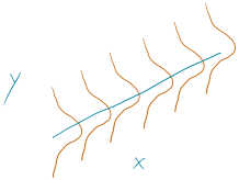
To make this clearer, suppose that in the Beers and BAC study that they had randomly assigned 20 students to consume each number of beers. We would expect some variation in the BAC for each group of 20 at each level of Beers but that each group of observations will be centered at the true mean BAC for each number of Beers. The regression model assumes that the BAC values are normally distributed around the mean for each Beer level, \(\text{BAC}_i \sim N(\beta_0 + \beta_1\text{ Beers}_i,\sigma^2)\), with the mean defined by the regression equation. We actually do not need to obtain more than one observation at each \(x\) value to make this assumption or assess it, but the plots below show you what this could look like. The sketch in Figure 7.1 attempts to show the idea of normal distributions that are centered at the true regression line, all with the same shape and variance that is an assumption of the regression model. Figure 7.2 contains simulated realizations from a normal distribution of 20 subjects at each Beer level around the assumed true regression line with two different residual SEs of 0.02 and 0.06. The original BAC model has a residual SE of 0.02 but had many fewer observations at each Beer value.

Figure 7.1: Sketch of assumed normal distributions for the responses centered at the regression line.

BB <- read_csv("http://www.math.montana.edu/courses/s217/documents/beersbac.csv")

Figure 7.2: Simulated data for Beers and BAC assuming two different residual standard errors (0.02 and 0.06).

Along with getting the idea that regression models define normal distributions in the y-direction that are centered at the regression line, you can also get a sense of how variable samples from a normal distribution can appear. Each distribution of 20 subjects at each \(x\) value came from a normal distribution but there are some of those distributions that might appear to generate small outliers and have slightly different variances. This can help us to remember to not be too particular when assessing assumptions and allow for some variability in spreads and a few observations from the tails of the distribution to occasionally arise.

In sampling from the population, we expect some amount of variability of each estimator around its true value. This variability leads to the potential variability in estimated regression lines (think of a suite of potential estimated regression lines that would be created by different random samples from the same population). Figure 7.3 contains the true regression line (bold, red) and realizations of the estimated regression line in simulated data based on results similar to the real data set. This variability due to random sampling is something that needs to be properly accounted for to use the single estimated regression line to make inferences about the true line and parameters based on the sample-based estimates. The next sections develop those inferential tools.

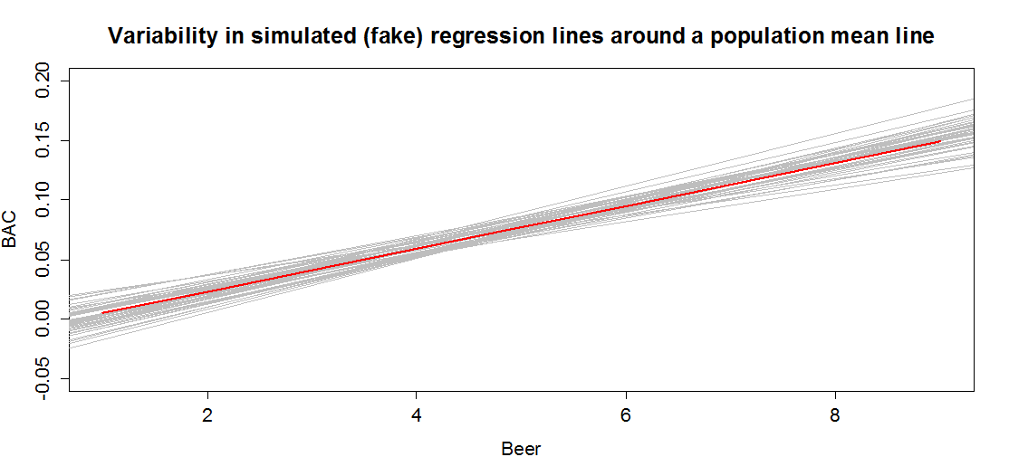
Figure 7.3: Variability in realized regression lines based on sampling variation. Light grey lines are simulated realizations assuming the bold (red) line is the true SLR model and variability is similar to the original BAC data set. Simulated observations from the estimated models using the simulate function as was used in Chapter 2 were used to create this plot.