7.2: Confidence interval and hypothesis tests for the slope and intercept

Our inference techniques will resemble previous material with an interest in forming confidence intervals and doing hypothesis testing, although the interpretation of confidence intervals for slope coefficients take some extra care. Remember that the general form of any parametric confidence interval is

\[\text{estimate} \mp t^*\text{SE}_{estimate},\]

so we need to obtain the appropriate standard error for regression model coefficients and the degrees of freedom to define the \(t\)-distribution to look up \(t^*\) multiplier. We will find the \(\text{SE}_{b_0}\) and \(\text{SE}_{b_1}\) in the model summary. The degrees of freedom for the \(t\)-distribution in simple linear regression are \(\mathbf{df = n-2}\). Putting this together, the confidence interval for the true y-intercept, \(\beta_0\), is \(\mathbf{b_0 \mp t^*_{n-2}}\textbf{SE}_{\mathbf{b_0}}\) although this confidence interval is rarely of interest. The confidence interval that is almost always of interest is for the true slope coefficient, \(\beta_1\), that is \(\mathbf{b_1 \mp t^*_{n-2}}\textbf{SE}_{\mathbf{b_1}}\). The slope confidence interval is used to do two things: (1) inference for the amount of change in the mean of \(y\) for a unit change in \(x\) in the population and (2) to potentially do hypothesis testing by checking whether 0 is in the CI or not. The sketch in Figure 7.4 illustrates the roles of the CI for the slope in terms of determining where the population slope, \(\beta_1\), coefficient might be – centered at the sample slope coefficient – our best guess for the true slope. This sketch also informs an interpretation of the slope coefficient confidence interval:

Figure 7.4: Graphic illustrating the confidence interval for a slope coefficient for a 1 unit increase in \(x\).

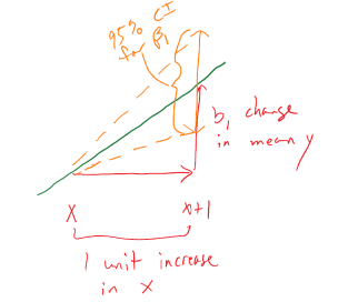
For a 1 [units of X] increase in X, we are ___ % confident that the true change in the mean of Y will be between LL and UL [units of Y].

In this interpretation, LL and UL are the calculated lower and upper limits of the confidence interval. This builds on our previous interpretation of the slope coefficient, adding in the information about pinning down the true change (population change) in the mean of the response variable for a difference of 1 unit in the \(x\)-direction. The interpretation of the y-intercept CI is:

For an x of 0 [units of X], we are 95% confident that the true mean of Y will be between LL and UL [units of Y].

This is really only interesting if the value of \(x = 0\) is interesting – we’ll see a method for generating CIs for the true mean at potentially more interesting values of \(x\) in Section 7.7. To trust the results from these confidence intervals, it is critical that any issues with the regression validity conditions are minor.

The only hypothesis test of interest in this situation is for the slope coefficient. To develop the hypotheses of interest in SLR, note the effect of having \(\beta_1 = 0\) in the mean of the regression equation, \(\mu_{y_i} = \beta_0 + \beta_1x_i = \beta_0 + 0x_i = \beta_0\). This is the “intercept-only” or “mean-only” model that suggests that the mean of \(y\) does not vary with different values of \(x\) as it is always \(\beta_0\). We saw this model in the ANOVA material as the reduced model when the null hypothesis of no difference in the true means across the groups was true. Here, this is the same as saying that there is no linear relationship between \(x\) and \(y\), or that \(x\) is of no use in predicting \(y\), or that we make the same prediction for \(y\) for every value of \(x\). Thus

\[\boldsymbol{H_0: \beta_1 = 0}\]

is a test for no linear relationship between \(\mathbf{x}\) and \(\mathbf{y}\) in the population. The alternative of \(\boldsymbol{H_A: \beta_1\ne 0}\), that there is some linear relationship between \(x\) and \(y\) in the population, is our main test of interest in these situations. It is also possible to test greater than or less than alternatives in certain situations.

Test statistics for regression coefficients are developed, if we can trust our assumptions, using the \(t\)-distribution with \(n-2\) degrees of freedom. The \(t\)-test statistic is generally

\[t = \frac{b_i}{\text{SE}_{b_i}}\]

with the main interest in the test for \(\beta_1\) based on \(b_1\) initially. The p-value would be calculated using the two-tailed area from the \(t_{n-2}\) distribution calculated using the pt function. The p-value to test these hypotheses is also provided in the model summary as we will see below.

The greater than or less than alternatives can have interesting interpretations in certain situations. For example, the greater than alternative \(\left(\boldsymbol{H_A: \beta_1 > 0}\right)\) tests an alternative of a positive linear relationship, with the p-value extracted just from the right tail of the same \(t\)-distribution. This could be used when a researcher would only find a result “interesting” if a positive relationship is detected, such as in the study of tree height and tree diameter where a researcher might be justified in deciding to test only for a positive linear relationship. Similarly, the left-tailed alternative is also possible, \(\boldsymbol{H_A: \beta_1 < 0}\). To get one-tailed p-values from two-tailed results (the default), first check that the observed test statistic is in the direction of the alternative (\(t>0\) for \(H_A:\beta_1>0\) or \(t<0\) for \(H_A:\beta_1<0\)). If these conditions are met, then the p-value for the one-sided test from the two-sided version is found by dividing the reported p-value by 2. If \(t>0\) for \(H_A:\beta_1>0\) or \(t<0\) for \(H_A:\beta_1<0\) are not met, then the p-value would be greater than 0.5 and it would be easiest to look it up directly using pt using the tail area direction in the direction of the alternative.

We can revisit a couple of examples for a last time with these ideas in hand to complete the analyses.

For the Beers, BAC data, the 95% confidence for the true slope coefficient, \(\beta_1\), is

\[\begin{array}{rl} \boldsymbol{b_1 \mp t^*_{n-2}} \textbf{SE}_{\boldsymbol{b_1}} & \boldsymbol{= 0.01796 \mp 2.144787 * 0.002402} \\ & \boldsymbol{= 0.01796 \mp 0.00515} \\ & \boldsymbol{\rightarrow (0.0128, 0.0231).} \end{array}\]

You can find the components of this calculation in the model summary and from qt(0.975, df = n-2) which was 2.145 for the \(t^*\)-multiplier. Be careful not to use the \(t\)-value of 7.48 in the model summary to make confidence intervals – that is the test statistic used below. The related calculations are shown at the bottom of the following code:

m1 <- lm(BAC ~ Beers, data = BB)
summary(m1)

## 
## Call:
## lm(formula = BAC ~ Beers, data = BB)
## 
## Residuals:
##       Min        1Q    Median        3Q       Max 
## -0.027118 -0.017350  0.001773  0.008623  0.041027 
## 
## Coefficients:
##              Estimate Std. Error t value Pr(>|t|)
## (Intercept) -0.012701   0.012638  -1.005    0.332
## Beers        0.017964   0.002402   7.480 2.97e-06
## 
## Residual standard error: 0.02044 on 14 degrees of freedom
## Multiple R-squared:  0.7998, Adjusted R-squared:  0.7855 
## F-statistic: 55.94 on 1 and 14 DF,  p-value: 2.969e-06

qt(0.975, df = 14) #t* multiplier for 95% CI

## [1] 2.144787

0.017964 + c(-1,1)*qt(0.975, df = 14)*0.002402

## [1] 0.01281222 0.02311578

qt(0.975, df = 14)*0.002402

## [1] 0.005151778

We can also get the confidence interval directly from the confint function run on our regression model, saving some calculation effort and providing both the CI for the y-intercept and the slope coefficient.

confint(m1)

##                   2.5 %     97.5 %
## (Intercept) -0.03980535 0.01440414
## Beers        0.01281262 0.02311490

We interpret the 95% CI for the slope coefficient as follows: For a 1 beer increase in number of beers consumed, we are 95% confident that the true change in the mean BAC will be between 0.0128 and 0.0231 g/dL. While the estimated slope is our best guess of the impacts of an extra beer consumed based on our sample, this CI provides information about the likely range of potential impacts on the mean in the population. It also could be used to test the two-sided hypothesis test and would suggest strong evidence against the null hypothesis since the confidence interval does not contain 0, but its main use is to quantify where we think the true slope coefficient resides.

The width of the CI, interpreted loosely as the precision of the estimated slope, is impacted by the variability of the observations around the estimated regression line, the overall sample size, and the positioning of the \(x\)-observations. Basically all those aspects relate to how “clearly” known the regression line is and that determines the estimated precision in the slope. For example, the more variability around the line that is present, the more uncertainty there is about the correct line to use (Least Squares (LS) can still find an estimated line but there are other lines that might be “close” to its optimizing choice). Similarly, more observations help us get a better estimate of the mean – an idea that permeates all statistical methods. Finally, the location of \(x\)-values can impact the precision in a slope coefficient. We’ll revisit this in the context of multicollinearity in the next chapter, and often we have no control of \(x\)-values, but just note that different patterns of \(x\)-values can lead to different precision of estimated slope coefficients¹²⁰.

For hypothesis testing, we will almost always stick with two-sided tests in regression modeling as it is a more conservative approach and does not require us to have an expectation of a direction for relationships a priori. In this example, the null hypothesis for the slope coefficient is that there is no linear relationship between Beers and BAC in the population. The alternative hypothesis is that there is some linear relationship between Beers and BAC in the population. The test statistic is \(t = 0.01796/0.002402 = 7.48\) which, if model assumptions hold, follows a \(t(14)\) distribution under the null hypothesis. The model summary provides the calculation of the test statistic and the two-sided test p-value of \(2.97\text{e-6} = 0.00000297\). So we would just report “p-value < 0.0001”. This suggests that there is very strong evidence against the null hypothesis of no linear relationship between Beers and BAC in the population, so we would conclude that there is a linear relationship between them. Because of the random assignment, we can also say that drinking beers causes changes in BAC but, because the sample was made up of volunteers, we cannot infer that these results would hold in the general population of OSU students or more generally.

There are also results for the y-intercept in the output. The 95% CI is from -0.0398 to 0.0144, that the true mean BAC for a 0 beer consuming subject is between -0.0398 to 0.01445. This is really not a big surprise but possibly is comforting to know that these results would not show much evidence against the null hypothesis that the true mean BAC for 0 Beers is 0. Finding little evidence of a difference from 0 makes sense and makes the estimated y-intercept of -0.013 not so problematic. In other situations, the results for the y-intercept may be more illogical but this will often be because the y-intercept is extrapolating far beyond the scope of observations. The y-intercept’s main function in regression models is to be at the right level for the slope to “work” to make a line that describes the responses and thus is usually of lesser interest even though it plays an important role in the model.

As a second example, we can revisit modeling the Hematocrit of female Australian athletes as a function of body fat %. The sample size is \(n = 99\) so the df are 97 in any \(t\)-distributions. In Chapter 6, the relationship between Hematocrit and body fat % for females appeared to be a weak negative linear association. The 95% confidence interval for the slope is -0.186 to 0.0155. For a 1% increase in body fat %, we are 95% confident that the change in the true mean Hematocrit is between -0.186 and 0.0155% of blood. This suggests that we would find little evidence against the null hypothesis of no linear relationship because this CI contains 0. In fact the p-value is 0.0965 which is larger than 0.05 and so provides a consistent conclusion with using the 95% confidence interval to perform a hypothesis test. Either way, we would conclude that there is not strong evidence against the null hypothesis but there is some evidence against it with a p-value of that size since more extreme results are somewhat common but still fairly rare if we assume the null is true. If you think p-values around 0.10 provide moderate evidence, you might have a different opinion about the evidence against the null hypothesis here. For this reason, we sometimes interpret this sort of marginal result as having some or marginal evidence against the null but certainly would never say that this presents strong evidence.

library(alr4)
data(ais)
library(tibble)
ais <- as_tibble(ais)
aisR <- ais %>% slice(-56, -166) #Removes observations in rows 56 and 166
m2 <- lm(Hc ~ Bfat, data = aisR %>% filter(Sex == 1)) #Results for Females 
summary(m2)

## 
## Call:
## lm(formula = Hc ~ Bfat, data = aisR %>% filter(Sex == 1))
## 
## Residuals:
##     Min      1Q  Median      3Q     Max 
## -5.2399 -2.2132 -0.1061  1.8917  6.6453 
## 
## Coefficients:
##             Estimate Std. Error t value Pr(>|t|)
## (Intercept) 42.01378    0.93269  45.046   <2e-16
## Bfat        -0.08504    0.05067  -1.678   0.0965
## 
## Residual standard error: 2.598 on 97 degrees of freedom
## Multiple R-squared:  0.02822,    Adjusted R-squared:  0.0182 
## F-statistic: 2.816 on 1 and 97 DF,  p-value: 0.09653

confint(m2)

##                  2.5 %      97.5 %
## (Intercept) 40.1626516 43.86490713
## Bfat        -0.1856071  0.01553165

One more worked example is provided from the Montana fire data. In this example pay particular attention to how we are handling the units of the response variable, log-hectares, and to the changes to doing inferences with a 99% confidence level CI, and where you can find the needed results in the following output:

mtfires <- read_csv("http://www.math.montana.edu/courses/s217/documents/climateR2.csv")

mtfires <- mtfires %>% mutate(loghectares = log(hectares))
fire1 <- lm(loghectares ~ Temperature, data = mtfires)
summary(fire1)

## 
## Call:
## lm(formula = loghectares ~ Temperature, data = mtfires)
## 
## Residuals:
##     Min      1Q  Median      3Q     Max 
## -3.0822 -0.9549  0.1210  1.0007  2.4728 
## 
## Coefficients:
##             Estimate Std. Error t value Pr(>|t|)
## (Intercept) -69.7845    12.3132  -5.667 1.26e-05
## Temperature   1.3884     0.2165   6.412 2.35e-06
## 
## Residual standard error: 1.476 on 21 degrees of freedom
## Multiple R-squared:  0.6619, Adjusted R-squared:  0.6458 
## F-statistic: 41.12 on 1 and 21 DF,  p-value: 2.347e-06

confint(fire1, level = 0.99)

##                    0.5 %     99.5 %
## (Intercept) -104.6477287 -34.921286
## Temperature    0.7753784   2.001499

qt(0.995, df = 21)

## [1] 2.83136

• Based on the estimated regression model, we can say that if the average temperature is 0, we expect that, on average, the log-area burned would be -69.8 log-hectares.
• From the regression model summary, \(b_1 = 1.39\) with \(\text{SE}_{b_1} = 0.2165\) and \(\mathbf{t = 6.41}\).
• There were \(n = 23\) measurements taken, so \(\mathbf{df = n-2 = 23-3 = 21}\).
• Suppose that we want to test for a linear relationship between temperature and log-hectares burned:

  \[H_0: \beta_1 = 0\]

  • In words, the true slope coefficient between Temperature and log-area burned is 0 OR there is no linear relationship between Temperature and log-area burned in the population.

  \[H_A: \beta_1\ne 0\]

  • In words, the alternative states that the true slope coefficient between Temperature and log-area burned is not 0 OR there is a linear relationship between Temperature and log-area burned in the population.

Test statistic: \(t = 1.39/0.217 = 6.41\)

• Assuming the null hypothesis to be true (no linear relationship), the \(t\)-statistic follows a \(t\)-distribution with \(n-2 = 23-2 = 21\) degrees of freedom (or simply \(t_{21}\)).

p-value:

• From the model summary, the p-value is \(\mathbf{2.35*10^{-6}}\)
  • Interpretation: There is less than a 0.01% chance that we would observe slope coefficient like we did or something more extreme (greater than 1.39 log(hectares)/\(^\circ F\)) if there were in fact no linear relationship between temperature (\(^\circ F\)) and log-area burned (log-hectares) in the population.

Conclusion: There is very strong evidence against the null hypothesis of no linear relationship, so we would conclude that there is, in fact, a linear relationship between Temperature and log(Hectares) burned.

Scope of Inference: Since we have a time series of results, our inferences pertain to the results we could have observed for these years but not for years we did not observe – so just for the true slope for this sample of years. Because we can’t randomly assign the amount of area burned, we cannot make causal inferences – there are many reasons why both the average temperature and area burned would vary together that would not involve a direct connection between them.

\[\text{99}\% \text{ CI for } \beta_1: \boldsymbol{b_1 \mp t^*_{n-2}}\textbf{SE}_{\boldsymbol{b_1}} \rightarrow 1.39 \mp 2.831\bullet 0.217 \rightarrow (0.78, 2.00)\]

Interpretation of 99% CI for slope coefficient:

• For a 1 degree F increase in Temperature, we are 99% confident that the change in the true mean log-area burned is between 0.78 and 2.00 log(Hectares).

Another way to interpret this is:

• For a 1 degree F increase in Temperature, we are 99% confident that the mean Area Burned will change by between 0.78 and 2.00 log(Hectares) in the population.

Also \(R^2\) is 66.2%, which tells us that Temperature explains 66.2% of the variation in log(Hectares) burned. Or that the linear regression model built using Temperature explains 66.2% of the variation in yearly log(Hectares) burned so this model explains quite a bit but not all the variation in the responses.