7.4: Randomization-based inferences for the slope coefficient

Exploring permutation testing in SLR provides an opportunity to gauge the observed relationship against the sorts of relationships we would expect to see if there was no linear relationship between the variables. If the relationship is linear (not curvilinear) and the null hypothesis of \(\beta_1 = 0\) is true, then any configuration of the responses relative to the predictor variable’s values is as good as any other. Consider the four scatterplots of the Bozeman temperature data versus Year and permuted versions of Year in Figure 7.8. First, think about which of the panels you think present the most evidence of a linear relationship between Year and Temperature?

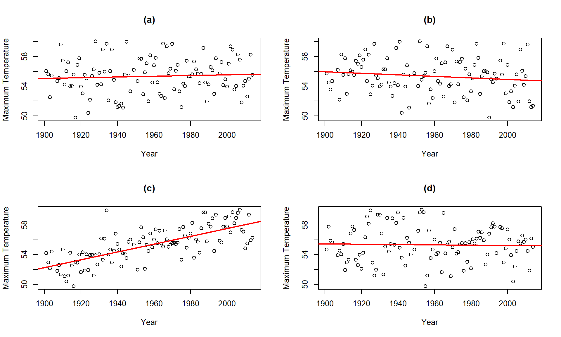
Figure 7.8: Plot of the Temperature responses versus four versions of Year, three of which are permutations of the Year variable relative to the Temperatures.

Hopefully you can see that panel (c) contains the most clear linear relationship among the choices. The plot in panel (c) is actually the real data set and pretty clearly presents itself as “different” from the other results. When we have small p-values, the real data set will be clearly different from the permuted results because it will be almost impossible to find a permuted data set that can attain as large a slope coefficient as was observed in the real data set¹²⁴. This result ties back into our original interests in this climate change research situation – does our result look like it is different from what could have been observed just by chance if there were no linear relationship between \(x\) and \(y\)? It seems unlikely…

Repeating this permutation process and tracking the estimated slope coefficients, as \(T^*\), provides another method to obtain a p-value in SLR applications. This could also be performed on the \(t\)-statistic for the slope coefficient and would provide the same p-values but the sampling distribution would have a different \(x\)-axis scaling. In this situation, the observed slope of 0.052 is really far from any possible values that can be obtained using permutations as shown in Figure 7.9. The p-value would be reported as \(<0.001\) for the two-sided permutation test.

Tobs <- lm(meanmax ~ Year, data = bozemantemps)$coef[2]
Tobs

##       Year 
## 0.05244213

B <- 1000
Tstar <- matrix(NA, nrow = B)

for (b in (1:B)){
  Tstar[b] <- lm(meanmax ~ shuffle(Year), data = bozemantemps)$coef[2]
}
pdata(abs(Tstar), abs(Tobs), lower.tail = F)[[1]]

## [1] 0

tibble(Tstar) %>%  ggplot(aes(x = Tstar)) + 
  geom_histogram(aes(y = ..ncount..), bins = 20, col = 1, fill = "skyblue") + 
  geom_density(aes(y = ..scaled..)) +
  theme_bw() +
  labs(y = "Density") +
  geom_vline(xintercept = c(-1,1)*Tobs, col = "red", lwd = 2) +
  stat_bin(aes(y = ..ncount.., label = ..count..), bins = 20,
           geom = "text", vjust = -0.75)

Figure 7.9: Permutation distribution of the slope coefficient in the Bozeman temperature linear regression model with bold vertical lines at \(\pm b_1 = 0.56\) based on the observed estimated slope.

One other interesting aspect of exploring the permuted data sets as in Figure 7.8 is that the outlier in the late 1930s “disappears” in the permuted data sets because there were many other observations that were that warm, just none that happened around that time of the century in the real data set. This reinforces the evidence for changes over time that seem to be present in these data – old unusual years don’t look unusual in more recent years (which is a pretty concerning result).

The permutation approach can be useful in situations where the normality assumption is compromised, but there are no influential points. In these situations, we might find more trustworthy p-values using permutations but only if we are working with an initial estimated regression equation that we generally trust. I personally like the permutation approach as a way of explaining what a p-value is actually measuring – the chance of seeing something like what we saw, or more extreme, if the null is true. And the previous scatterplots show what the “by chance” versions of this relationship might look like.

In a similar situation where we want to focus on confidence intervals for slope coefficients but are not completely comfortable with the normality assumption, it is also possible to generate bootstrap confidence intervals by sampling with replacement from the data set. This idea was introduced in Sections 2.8 and 2.9. This provides a 95% bootstrap confidence interval from 0.0433 to 0.061, which almost exactly matches the parametric \(t\)-based confidence interval. The bootstrap distributions are very symmetric (Figure 7.10). The interpretation is the same and this result reinforces the other assessments that the parametric approach is not unreasonable here except possibly for the independence assumption. These randomization approaches provide no robustness against violations of the independence assumption.

Tobs <- lm(meanmax ~ Year, data = bozemantemps)$coef[2]
Tobs

##       Year 
## 0.05244213

B <- 1000
Tstar <- matrix(NA, nrow = B)
for (b in (1:B)){
  Tstar[b] <- lm(meanmax ~ Year, data = resample(bozemantemps))$coef[2]
}
quantiles <- qdata(Tstar, c(0.025, 0.975))
quantiles

##       2.5%      97.5% 
## 0.04326952 0.06131044

tibble(Tstar) %>%  ggplot(aes(x = Tstar)) + 
  geom_histogram(aes(y = ..ncount..), bins = 15, col = 1, fill = "skyblue", center = 0) + 
  geom_density(aes(y = ..scaled..)) +
  theme_bw() +
  labs(y = "Density") +
  geom_vline(xintercept = quantiles, col = "blue", lwd = 2, lty = 3) +    
  geom_vline(xintercept = Tobs, col = "red", lwd = 2) +
  stat_bin(aes(y = ..ncount.., label = ..count..), bins = 15,
           geom = "text", vjust = -0.75)

Figure 7.10: Bootstrap distribution of the slope coefficient in the Bozeman temperature linear regression model with bold dashed vertical lines delineating the 95% confidence interval and the bold solid line the observed slope of 0.052.