5.10: Is cheating and lying related in students?

Last updated
Save as PDF

Page ID: 33258

$ \newcommand{\vecs}[1]{\overset { \scriptstyle \rightharpoonup} {\mathbf{#1}} } $ $ \newcommand{\vecd}[1]{\overset{-\!-\!\rightharpoonup}{\vphantom{a}\smash {#1}}} $$\newcommand{\id}{\mathrm{id}}$ $ \newcommand{\Span}{\mathrm{span}}$ $ \newcommand{\kernel}{\mathrm{null}\,}$ $ \newcommand{\range}{\mathrm{range}\,}$ $ \newcommand{\RealPart}{\mathrm{Re}}$ $ \newcommand{\ImaginaryPart}{\mathrm{Im}}$ $ \newcommand{\Argument}{\mathrm{Arg}}$ $ \newcommand{\norm}[1]{\| #1 \|}$ $ \newcommand{\inner}[2]{\langle #1, #2 \rangle}$ $ \newcommand{\Span}{\mathrm{span}}$ $\newcommand{\id}{\mathrm{id}}$ $ \newcommand{\Span}{\mathrm{span}}$ $ \newcommand{\kernel}{\mathrm{null}\,}$ $ \newcommand{\range}{\mathrm{range}\,}$ $ \newcommand{\RealPart}{\mathrm{Re}}$ $ \newcommand{\ImaginaryPart}{\mathrm{Im}}$ $ \newcommand{\Argument}{\mathrm{Arg}}$ $ \newcommand{\norm}[1]{\| #1 \|}$ $ \newcommand{\inner}[2]{\langle #1, #2 \rangle}$ $ \newcommand{\Span}{\mathrm{span}}$$\newcommand{\AA}{\unicode[.8,0]{x212B}}$

A study of student behavior was performed at a university with a survey of $N = 319$ undergraduate students (cheating data set from the poLCA package originally published by Dayton (1998)). They were asked to answer four questions about their various academic frauds that involved cheating and lying. Specifically, they were asked if they had ever lied to avoid taking an exam (LIEEXAM with 1 for no and 2 for yes), if they had lied to avoid handing in a term paper on time (LIEPAPER with 1 for no, 2 for yes), if they had purchased a term paper to hand in as their own or obtained a copy of an exam prior to taking the exam (FRAUD with 1 for no, 2 for yes), and if they had copied answers during an exam from someone near them (COPYEXAM with 1 for no, 2 for yes). Additionally, their GPAs were obtained and put into categories: (<2.99, 3.0 to 3.25, 3.26 to 3.50, 3.51 to 3.75, and 3.76 to 4.0). These categories were coded from 1 to 5, respectively. Again, the code starts with making sure the variables are treated categorically by applying the factor function.

library(poLCA)
data(cheating) #Survey of students
cheating <- as_tibble(cheating)

cheating <- cheating %>% mutate(LIEEXAM = factor(LIEEXAM),
                                LIEPAPER = factor(LIEPAPER),
                                FRAUD = factor(FRAUD),
                                COPYEXAM = factor(COPYEXAM),
                                GPA = factor(GPA)
                                )

tableplot(cheating, sort = GPA, pals = list("BrBG"))

Figure 5.18: Tableplot of initial cheating and lying data set. Note that a few GPAs were missing in the data set.

We can explore some interesting questions about the relationships between these variables. The tableplot in Figure 5.18 again helps us to get a general idea of the data set and to assess some complicated aspects of the relationships between variables. For example, the rates of different unethical behaviors seem to decrease with higher GPA students (but do not completely disappear!). This data set also has a few missing GPAs that we would want to carefully consider – which sorts of students might not be willing to reveal their GPAs? It ends up that these students did not admit to any of the unethical behaviors… Note that we used the sort = GPA option in the tableplot function to sort the responses based on GPA to see how GPA might relate to patterns of unethical behavior.

While the relationship between GPA and presence/absence of the different behaviors is of interest, we want to explore the types of behaviors. It is possible to group the lying behaviors as being a different type (less extreme?) of unethical behavior than obtaining an exam prior to taking it, buying a paper, or copying someone else’s answers. We want to explore whether there is some sort of relationship between the lying and copying behaviors – are those that engage in one type of behavior more likely to do the other? Or are they independent of each other? This is a hard story to elicit from the previous plot because there are so many variables involved.

Tableplot of new variables liar and copier that allow exploration of relationships between different types of lying and cheating behaviors. — Figure 5.19: Tableplot of new variables `liar` and `copier` that allow exploration of relationships between different types of lying and cheating behaviors.

To simplify the results, combining the two groups of variables into the four possible combinations on each has the potential to simplify the results – or at least allow exploration of additional research questions. The interaction function is used to create two new variables that have four levels that are combinations of the different options from none to both of each type (copier and liar). In the tableplot in Figure 5.19, you can see the four categories for each, starting with no bad behavior of either type (which is fortunately the most popular response on both variables!). For each variable, there are students who admitted to one of the two violations and some that did both. The liar variable has categories of None, ExamLie, PaperLie, and LieBoth. The copier variable has categories of None, PaperCheat, ExamCheat, and PaperExamCheat (for doing both). The last category for copier seems to mostly occur at the top of the plot which is where the students who had lied to get out of things reside, so maybe there is a relationship between those two types of behaviors? On the other hand, for the students who have never lied, quite a few had cheated on exams. The contingency table can help us dig further into the hypotheses related to the Chi-square test of Independence that is appropriate in this situation.

cheating <- cheating %>% mutate(liar = interaction(LIEEXAM, LIEPAPER),
                                copier = interaction(FRAUD, COPYEXAM)
                                )
levels(cheating$liar) <- c("None", "ExamLie", "PaperLie", "LieBoth")
levels(cheating$copier) <- c("None", "PaperCheat", "ExamCheat", "PaperExamCheat")

tableplot(cheating, sort = liar, select = c(liar, copier), pals = list("BrBG"))

cheatlietable <- tally(~ liar + copier, data = cheating)
cheatlietable

##           copier
## liar       None PaperCheat ExamCheat PaperExamCheat
##   None      207          7        46              5
##   ExamLie    10          1         3              2
##   PaperLie   13          1         4              2
##   LieBoth    11          1         4              2

Unfortunately for our statistic, there were very few responses in some combinations of categories even with $N = 319$. For example, there was only one response each in the combinations for students that copied on papers and lied to get out of exams, papers, and both. Some other categories were pretty small as well in the groups that only had one behavior present. To get a higher number of counts in the combinations, we combined the single behavior only levels into “either” categories and left the none and both categories for each variable. This creates two new variables called liar2 and copier2 (tableplot in Figure 5.20). The code to create these variables and make the plot is below which employs the levels function to assign the same label to two different levels from the original list.

# Collapse the middle categories of both variables by making both have the same level name:
cheating <- cheating %>% mutate(liar2 = liar, 
                                copier2 = copier
                                )
levels(cheating$liar2) <- c("None", "ExamorPaper", "ExamorPaper", "LieBoth")
levels(cheating$copier2) <- c("None", "ExamorPaper", "ExamorPaper", "CopyBoth")
tableplot(cheating, sort = liar2, select = c(liar2, copier2), pals = list("BrBG"))

Figure 5.20: Tableplot of lying and copying variables after combining categories.

cheatlietable <- tally(~ liar2 + copier2, data = cheating)
cheatlietable

##              copier2
## liar2         None ExamorPaper CopyBoth
##   None         207          53        5
##   ExamorPaper   23           9        4
##   LieBoth       11           5        2

This $3\times 3$ table is more manageable and has few really small cells so we will proceed with the 6+ steps of hypothesis testing applied to these data using the Independence testing methods (again a single sample was taken from the population so that is the appropriate procedure to employ):

The RQ is about relationships between lying to instructors and cheating and these questions, after some work and simplifications, allow us to address a version of that RQ even though it might not be the one that we started with. The tableplots help to visualize the results and the $X^2$-statistic will be used to do the hypothesis test.
Hypotheses:
- $H_0$: Lying and copying behavior are independent in the population of students at this university.
- $H_A$: Lying and copying behavior are dependent in the population of students at this university.
Validity conditions:
- Independence:
  - There is no indication of a violation of this assumption since each subject is measured only once in the table. No other information suggests a potential issue but we don’t have much information on how these subjects were obtained. What happens if we had sampled from students in different sections of a multi-section course and one of the sections had recently had a cheating scandal that impacted many students in that section?
- All expected cell counts larger than 5 (required to use $\chi^2$-distribution to find p-values):
  - We need to generate a table of expected cell counts to check this condition:
```
chisq.test(cheatlietable)$expected
```
```
##              copier2
## liar2              None ExamorPaper  CopyBoth
##   None        200.20376   55.658307 9.1379310
##   ExamorPaper  27.19749    7.561129 1.2413793
##   LieBoth      13.59875    3.780564 0.6206897
```
  - When we request the expected cell counts, there is a warning message (not shown).
  - There are three expected cell counts below 5, so the condition is violated and a permutation approach should be used to obtain more trustworthy p-values.
Calculate the test statistic and p-value:
- Use chisq.test to obtain the test statistic, although this table is small enough to do by hand if you want the practice – see if you can find a similar answer to what the function provides:
```
chisq.test(cheatlietable)
```
```
## 
##  Pearson's Chi-squared test
## 
## data:  cheatlietable
## X-squared = 13.238, df = 4, p-value = 0.01017
```
- The $X^2$ statistic is 13.24.
- The parametric p-value is 0.0102 from the R output. This was based on a $\chi^2$-distribution with $(3-1)*(3-1) = 4$ degrees of freedom that is displayed in Figure 5.21. Remember that this isn’t quite the right distribution for the test statistic since our expected cell count condition was violated.
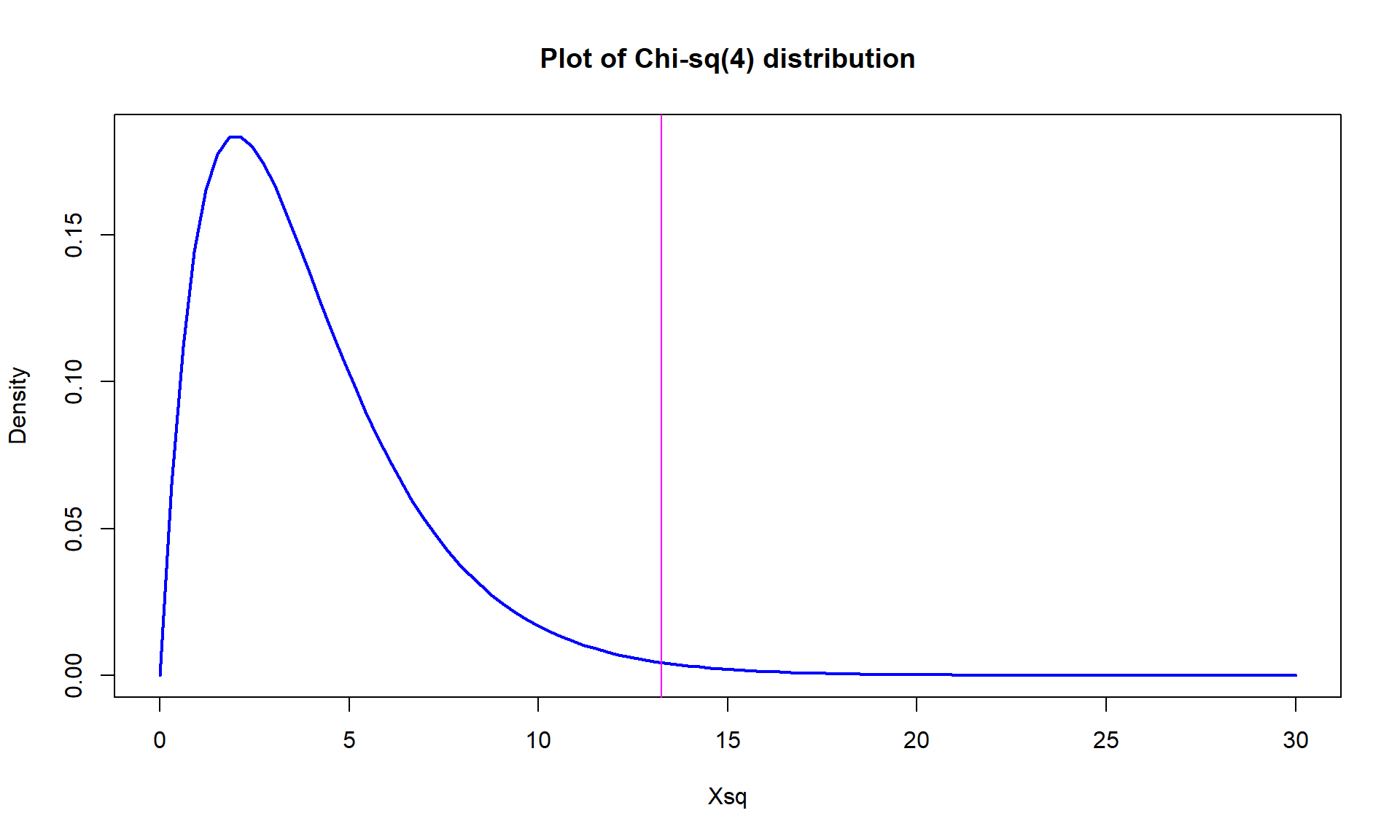
$Plot of $\boldsymbol{\chi^2}$-distribution with 4 degrees of freedom.$
Figure 5.21: Plot of $\boldsymbol{\chi^2}$-distribution with 4 degrees of freedom.
- If you want to repeat the p-value calculation directly:
```
pchisq(13.2384, df = 4, lower.tail = F)
```
```
## [1] 0.01016781
```
- But since the expected cell condition is violated, we should use permutations as implemented in the following code with the number of permutations increased to 10,000 to help get a better estimate of the p-value since it is possibly close to 0.05:
```
Tobs <- chisq.test(tally(~ liar2 + copier2, data = cheating))$statistic
Tobs
```
```
## X-squared 
##  13.23844
```
```
par(mfrow = c(1,2))
B <- 10000 # Now performing 10,000 permutations
Tstar <- matrix(NA,nrow = B)
for (b in (1:B)){
  Tstar[b] <- chisq.test(tally(~ shuffle(liar2) + copier2,
                               data = cheating))$statistic
}
pdata(Tstar, Tobs, lower.tail = F)[[1]]
```
```
## [1] 0.0174
```
```
tibble(Tstar) %>%  ggplot(aes(x = Tstar)) + 
  geom_histogram(aes(y = ..ncount..), bins = 20, col = 1, fill = "khaki") + 
  geom_density(aes(y = ..scaled..)) +
  theme_bw() +
  labs(y = "Density") +
  geom_vline(xintercept = Tobs, col = "red", lwd = 2) +
  stat_bin(aes(y = ..ncount.., label = ..count..), bins = 20,
           geom = "text", vjust = -0.75)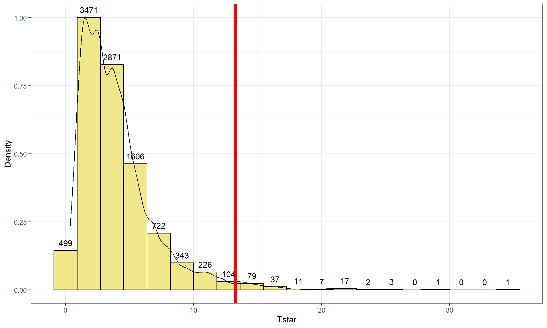
```
Figure 5.22: Plot of permutation distributions for cheat/lie results with observed value of 13.24 (bold, vertical line).
- There were 174 of $B$ = 10,000 permuted data sets that produced as large or larger $X^{2*}\text{'s}$ than the observed as displayed in Figure 5.22, so we report that the p-value was 0.0174 using the permutation approach, which was slightly larger than the result provided by the parametric method.
Conclusion:
- There is strong evidence against the null hypothesis of no relationship between lying and copying behavior in the population of students ($X^2$-statistic = 13.24, permutation p-value of 0.0174), so conclude that there is a relationship between lying and copying behavior at the university in the population of students studied.

Size:
- The standardized residuals can help us more fully understand this result – the mosaic plot only had one cell shaded and so wasn’t needed here.
```
chisq.test(cheatlietable)$residuals
```
```
##              copier2
## liar2               None ExamorPaper   CopyBoth
##   None         0.4803220  -0.3563200 -1.3688609
##   ExamorPaper -0.8048695   0.5232734  2.4759378
##   LieBoth     -0.7047165   0.6271633  1.7507524
```
- There is really only one large standardized residual for the ExamorPaper liars and the CopyBoth copiers, with a much larger observed value than expected of 2.48. The only other medium-sized standardized residuals came from the CopyBoth copiers column with fewer than expected students in the None category and more than expected in the LieBoth type of lying category. So we are seeing more than expected that lied somehow and copied – we can say this suggests that the students who lie tend to copy too!
Scope of inference:
- There is no causal inference possible here since neither variable was randomly assigned (really neither is explanatory or response here either) but we can extend the inferences to the population of students that these were selected from that would be willing to reveal their GPA (see initial discussion related to some differences in students that wouldn’t answer that question).