5.11: Analyzing a stratified random sample of California schools

Figure 5.23: Pirate-plot of the API growth scores by level of school in the stype variable (coded E for elementary, M for Middle, and H for High school).

In recent decades, there has been a push for quantification of school performance and tying financial punishment and rewards to growth in these metrics both for schools and for teachers. One example is the API (Academic Performance Index) in California that is based mainly on student scores on standardized tests. It ranges between 200 and 1000 and year to year changes are of interest to assess “performance” of schools – calculated as one year minus the previous year (negative “growth” is also possible!). Suppose that a researcher is interested in whether the growth metric might differ between different levels of schools. Maybe it is easier or harder for elementary, middle, or high schools to attain growth? The researcher has a list of most of the schools in the state of each level that are using a database that the researcher has access to. In order to assess this question, the researcher takes a stratified random sample¹⁰⁷, selecting \(n_{\text{elementary}} = 100\) schools from the population of 4421 elementary schools, \(n_{\text{middle}} = 50\) from the population of 1018 middle schools, and \(n_{\text{high}} = 50\) from the population of 755 high schools. These data are available in the survey package (Lumley 2021) and the api data object that loads both apipop (population) and apistrat (stratified random sample) data sets. The growth (change!) in API scores for the schools between 1999 and 2000 (taken as the year 2000 score minus 1999 score) is used as the response variable. The pirate-plot of the growth scores are displayed in Figure 5.23. They suggest some differences in the growth rates among the different levels. There are also a few schools flagged as being possible outliers.

library(survey)
data(api)
apistrat <- as_tibble(apistrat)
apipop <- as_tibble(apipop)
tally(~ stype, data = apipop) #Population counts

## stype
##    E    H    M 
## 4421  755 1018

tally(~ stype, data = apistrat) #Sample counts

## stype
##   E   H   M 
## 100  50  50

pirateplot(growth ~ stype, data = apistrat, inf.method = "ci", inf.disp = "line")

The One-Way ANOVA \(F\)-test, provided below, suggests strong evidence against the null hypothesis of no difference in the true mean growth scores among the different types of schools (\(F(2,197) = 23.56\), \(\text{ p-value}<0.0001\)). But the residuals from this model displayed in the QQ-Plot in Figure 5.24 contain a slightly long right tail and short left tail, suggesting a right skewed distribution for the residuals. In a high-stakes situation such as this, reporting results with violations of the assumptions probably would not be desirable, so another approach is needed. The permutation methods would be justified here but there is another “simpler” option available using our new Chi-square analysis methods.

m1 <- lm(growth ~ stype, data = apistrat)
library(car)
Anova(m1)

## Anova Table (Type II tests)
## 
## Response: growth
##           Sum Sq  Df F value    Pr(>F)
## stype      30370   2  23.563 6.685e-10
## Residuals 126957 197

plot(m1, which = 2, pch = 16)

Figure 5.24: QQ-plot of standardized residuals from the One-Way ANOVA linear model.

One way to get around the normality assumption is to use a method that does not assume the responses follow a normal distribution. If we bin or cut the quantitative response variable into a set of ordered categories and apply a Chi-square test, we can proceed without concern about the lack of normality in the residuals of the ANOVA model. To create these bins, a simple idea would be to use the quartiles to generate the response variable categories, binning the quantitative responses into groups for the lowest 25%, second 25%, third 25%, and highest 25% by splitting the data at \(Q_1\), the Median, and \(Q_3\). In R, the cut function is available to turn a quantitative variable into a categorical variable. First, we can use the information from favstats to find the cut-points:

favstats(~ growth, data = apistrat)

##  min   Q1 median Q3 max   mean      sd   n missing
##  -47 6.75     25 48 133 27.995 28.1174 200       0

The cut function can provide the binned variable if it is provided with the end-points of the desired intervals (breaks = ...) to create new categories with those names in a new variable called growthcut.

apistrat <- apistrat %>% mutate(growthcut = cut(growth, breaks = c(-47,6.75,25,48,133),
                                                include.lowest = T))

tally(~ growthcut, data = apistrat)

## growthcut
## [-47,6.75]  (6.75,25]    (25,48]   (48,133] 
##         50         52         49         49

Now that we have a categorical response variable, we need to decide which sort of Chi-square analysis to perform. The sampling design determines the correct analysis as always in these situations. The stratified random sample involved samples from each of the three populations so a Homogeneity test should be employed. In these situations, the stacked bar chart provides the appropriate summary of the data. It also shows us the labels of the categories that the cut function created in the new growthcut variable:

Figure 5.25: Stacked bar chart of the growth category responses by level of school.

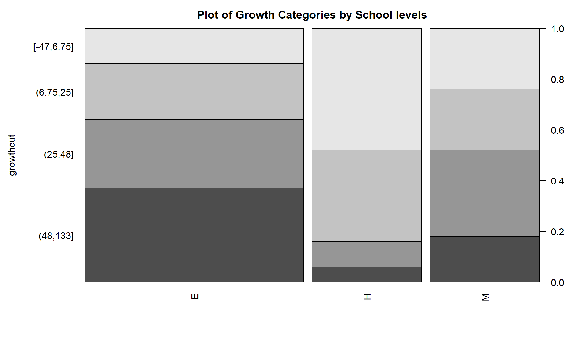
plot(growthcut ~ stype, data = apistra, 
     main = "Plot of Growth Categories by School levels")

Figure 5.25 suggests that the distributions of growth scores may not be the same across the levels of the schools with many more high growth Elementary schools than in either the Middle or High school groups (the “high” growth category is labeled as (48, 133] providing the interval of growth scores placed in this category). Similarly, the proportion of the low or negative growth (category of (-47.6, 6.75] for “growth” between -47.6 and 6.75) is least frequently occurring in Elementary schools and most frequent in the High schools. Statisticians often work across many disciplines and so may not always have the subject area knowledge to know why these differences exist (just like you might not), but an education researcher could take this sort of information – because it is a useful summary of interesting school-level data – and generate further insights into why growth in the API metric may or may not be a good or fair measure of school performance.

Of course, we want to consider whether these results can extend to the population of all California schools. The homogeneity hypotheses for assessing the growth rate categories across the types of schools would be:

• \(H_0\): There is no difference in the distribution of growth categories across the three levels of schools in the population of California schools.
• \(H_A\): There is some difference in the distribution of growth categories across the three levels of schools in the population of California schools.

There might be an issue with the independence assumption in that schools within the same district might be more similar to one another and different between one another. Sometimes districts are accounted for in education research to account for differences in policies and demographics among the districts. We could explore this issue by finding district-level average growth rates and exploring whether those vary systematically but this is beyond the scope of the current exploration.

Checking the expected cell counts gives insight into the assumption for using the \(\boldsymbol{\chi^2}\)-distribution to find the p-value:

growthtable <- tally(~ stype + growthcut, data = apistrat)
growthtable

##      growthcut
## stype [-47,6.75] (6.75,25] (25,48] (48,133]
##     E         14        22      27       37
##     H         24        18       5        3
##     M         12        12      17        9

chisq.test(growthtable)$expected 

##      growthcut
## stype [-47,6.75] (6.75,25] (25,48] (48,133]
##     E       25.0        26   24.50    24.50
##     H       12.5        13   12.25    12.25
##     M       12.5        13   12.25    12.25

The smallest expected count is 12.25, occurring in four different cells, so we can use the parametric approach.

chisq.test(growthtable) 

## 
##  Pearson's Chi-squared test
## 
## data:  growthtable
## X-squared = 38.668, df = 6, p-value = 8.315e-07

The observed test statistic is \(X^2 = 38.67\) and, based on a \(\boldsymbol{\chi^2}(6)\) distribution, the p-value is 0.0000008. This p-value suggests that there is very strong evidence against the null hypothesis of no difference in the distribution of API growth of schools among Elementary, Middle and High School in the population of schools in California between 1999 and 2000, and we can conclude that there is some difference in the population (California schools). Because the schools were randomly selected from all the California schools we can make valid inferences to all the schools but because the level of schools, obviously, cannot be randomly assigned, we cannot say that level of school causes these differences.

The standardized residuals can enhance this interpretation, displayed in Figure 5.26. The Elementary schools have fewer low/negative growth schools and more high growth schools than expected under the null hypothesis. The High schools have more low growth and fewer higher growth (growth over 25 points) schools than expected if there were no difference in patterns of response across the school levels. The Middle school results were closer to the results expected if there were no differences across the school levels.

chisq.test(growthtable)$residuals

##      growthcut
## stype [-47,6.75]  (6.75,25]    (25,48]   (48,133]
##     E -2.2000000 -0.7844645  0.5050763  2.5253814
##     H  3.2526912  1.3867505 -2.0714286 -2.6428571
##     M -0.1414214 -0.2773501  1.3571429 -0.9285714

Figure 5.26: Mosaic plot of the API Growth rate categories versus level of the school with shading for size of standardized residuals.

mosaicplot(growthcut ~ stype, data = apistrat, shade = T)

The binning of quantitative variables is not a first step in analyses – the quantitative version is almost always preferable. However, this analysis avoided the violation of the normality assumption that was somewhat problematic for the ANOVA and still provided useful inferences to the differences in the types of schools. When one goes from a quantitative to categorical version of a variable, one loses information (the specific details of the quantitative responses within each level created) and this almost always will result in a loss of statistical power of the procedure. In this situation, the p-value from the ANOVA was of the order \(10^{-10}\) while the Chi-square test had a p-value of order \(10^{-7}\). This larger p-value is typical of the loss of power in going to a categorical response when more information was available. In many cases, there are no options but to use contingency table analyses. This example shows that there might be some situations where “going categorical” could be an acceptable method for handing situations where an assumption is violated.