2.6: Connecting randomization (nonparametric) and parametric tests

Last updated
Save as PDF

Page ID: 33219

$ \newcommand{\vecs}[1]{\overset { \scriptstyle \rightharpoonup} {\mathbf{#1}} } $ $ \newcommand{\vecd}[1]{\overset{-\!-\!\rightharpoonup}{\vphantom{a}\smash {#1}}} $$\newcommand{\id}{\mathrm{id}}$ $ \newcommand{\Span}{\mathrm{span}}$ $ \newcommand{\kernel}{\mathrm{null}\,}$ $ \newcommand{\range}{\mathrm{range}\,}$ $ \newcommand{\RealPart}{\mathrm{Re}}$ $ \newcommand{\ImaginaryPart}{\mathrm{Im}}$ $ \newcommand{\Argument}{\mathrm{Arg}}$ $ \newcommand{\norm}[1]{\| #1 \|}$ $ \newcommand{\inner}[2]{\langle #1, #2 \rangle}$ $ \newcommand{\Span}{\mathrm{span}}$ $\newcommand{\id}{\mathrm{id}}$ $ \newcommand{\Span}{\mathrm{span}}$ $ \newcommand{\kernel}{\mathrm{null}\,}$ $ \newcommand{\range}{\mathrm{range}\,}$ $ \newcommand{\RealPart}{\mathrm{Re}}$ $ \newcommand{\ImaginaryPart}{\mathrm{Im}}$ $ \newcommand{\Argument}{\mathrm{Arg}}$ $ \newcommand{\norm}[1]{\| #1 \|}$ $ \newcommand{\inner}[2]{\langle #1, #2 \rangle}$ $ \newcommand{\Span}{\mathrm{span}}$$\newcommand{\AA}{\unicode[.8,0]{x212B}}$

In developing statistical inference techniques, we need to define the test statistic, $T$, that measures the quantity of interest. To compare the means of two groups, a statistic is needed that measures their differences. In general, for comparing two groups, the choice is simple – a difference in the means often works well and is a natural choice. There are other options such as tracking the ratio of means or possibly the difference in medians. Instead of just using the difference in the means, we also could “standardize” the difference in the means by dividing by an appropriate quantity that reflects the variation in the difference in the means. All of these are valid and can sometimes provide similar results – it ends up that there are many possibilities for testing using the randomization (nonparametric) techniques introduced previously. Parametric statistical methods focus on means because the statistical theory surrounding means is quite a bit easier (not easy, just easier) than other options. There are just a couple of test statistics that you can use and end up with named distributions to use for generating inferences. Randomization techniques allow inference for other quantities (such as ratios of means or differences in medians) but our focus here will be on using randomization for inferences on means to see the similarities with the more traditional parametric procedures used in these situations.

In two-sample mean situations, instead of working just with the difference in the means, we often calculate a test statistic that is called the equal variance two-independent samples t-statistic. The test statistic is

\[t = \frac{\bar{x}_1 - \bar{x}_2}{s_p\sqrt{\frac{1}{n_1}+\frac{1}{n_2}}},\]

where $s_1^2$ and $s_2^2$ are the sample variances for the two groups, $n_1$ and $n_2$ are the sample sizes for the two groups, and the pooled sample standard deviation,

\[s_p = \sqrt{\frac{(n_1-1)s_1^2 + (n_2-1)s_2^2}{n_1+n_2-2}}.\]

The $t$-statistic keeps the important comparison between the means in the numerator that we used before and standardizes (re-scales) that difference so that $t$ will follow a $t$-distribution (a parametric “named” distribution) if certain assumptions are met. But first we should see if standardizing the difference in the means had an impact on our permutation test results. It ends up that, while not too obvious, the summary of the lm we fit earlier contains this test statistic⁴³. Instead of using the second model coefficient that estimates the difference in the means of the groups, we will extract the test statistic from the table of summary output that is in the coef object in the summary – using $ to reference the coef information only. In the coef object in the summary, results related to the ConditionCommute are again useful for the comparison of two groups.

summary(lm1)$coef

##                   Estimate Std. Error   t value     Pr(>|t|)
## (Intercept)      135.80000   8.862996 15.322133 3.832161e-15
## Conditioncommute -25.93333  12.534169 -2.069011 4.788928e-02

The first column of numbers contains the estimated difference in the sample means (-25.933 here) that was used before. The next column is the Std. Error column that contains the standard error (SE) of the estimated difference in the means, which is $s_p\sqrt{\frac{1}{n_1}+\frac{1}{n_2}}$ and also the denominator used to form the $t$-test statistic (12.53 here). It will be a common theme in this material to take the ratio of the estimate (-25.933) to its SE (12.53) to generate test statistics, which provides -2.07 – this is the “standardized” estimate of the difference in the means. It is also a test statistic ($T$) that we can use in a permutation test. This value is in the second row and third column of summary(lm1)$coef and to extract it the bracket notation is again employed. Specifically we want to extract summary(lm1)$coef[2,3] and using it and its permuted data equivalents to calculate a p-value. Since we are doing a two-sided test, the code resembles the permutation test code in Section 2.4 with the new $t$-statistic replacing the difference in the sample means that we used before.

Tobs <- summary(lm1)$coef[2,3]
Tobs

## [1] -2.069011

B <- 1000
set.seed(406)
Tstar <- matrix(NA, nrow = B)
for (b in (1:B)){
  lmP <- lm(Distance ~ shuffle(Condition), data = dsample)
  Tstar[b] <- summary(lmP)$coef[2,3]
}
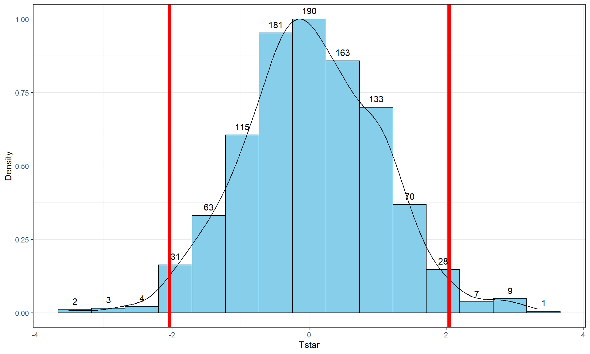
pdata(abs(Tstar), abs(Tobs), lower.tail = F)

## [1] 0.041

The permutation distribution in Figure 2.12 looks similar to the previous results with slightly different $x$-axis scaling. The observed $t$-statistic was $-2.07$ and the proportion of permuted results that were as or more extreme than the observed result was 0.041. This difference is due to a different set of random permutations being selected. If you run permutation code, you will often get slightly different results each time you run it. If you are uncomfortable with the variation in the results, you can run more than B = 1,000 permutations (say 10,000) and the variability in the resulting p-values will be reduced further. Usually this uncertainty will not cause any substantive problems – but do not be surprised if your results vary if you use different random number seeds.

Figure 2.12: Permutation distribution of the $t$-statistic.

tibble(Tstar) %>% ggplot(aes(x = Tstar)) + 
  geom_histogram(aes(y = ..ncount..), bins = 15, col = 1, fill = "skyblue", center = 0) + 
  geom_density(aes(y = ..scaled..)) +
  theme_bw() +
  labs(y = "Density") +
  geom_vline(xintercept = c(-1,1)*Tobs, col = "red", lwd = 2) +
  stat_bin(aes(y = ..ncount.., label = ..count..), bins = 15, 
           geom = "text", vjust = -0.75)

The parametric version of these results is based on using what is called the two-independent sample t-test. There are actually two versions of this test, one that assumes that variances are equal in the groups and one that does not. There is a rule of thumb that if the ratio of the larger standard deviation over the smaller standard deviation is less than 2, the equal variance procedure is OK. It ends up that this assumption is less important if the sample sizes in the groups are approximately equal and more important if the groups contain different numbers of observations. In comparing the two potential test statistics, the procedure that assumes equal variances has a complicated denominator (see the formula above for $t$ involving $s_p$) but a simple formula for degrees of freedom (df) for the $t$-distribution ($df = n_1+n_2-2$) that approximates the distribution of the test statistic, $t$, under the null hypothesis. The procedure that assumes unequal variances has a simpler test statistic and a very complicated degrees of freedom formula. The equal variance procedure is equivalent to the methods we will consider in Chapters 3 and 4 so that will be our focus for the two group problem and is what we get when using the lm model to estimate the differences in the group means. The unequal variance version of the two-sample t-test is available in the t.test function if needed.

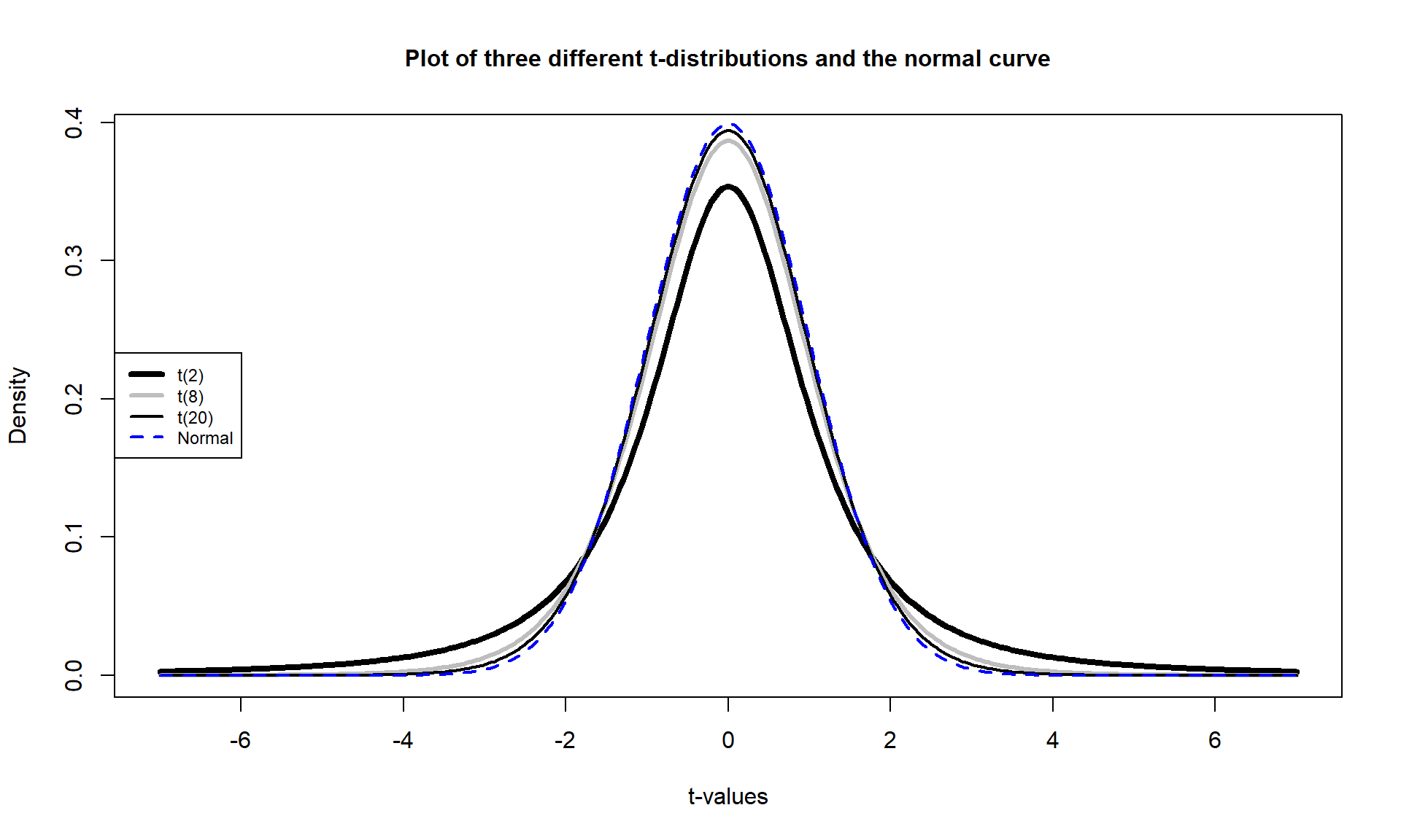
Plots of $t$-distributions with 2, 8, and 20 degrees of freedom and a normal distribution (dashed line). Note how the $t$-distributions get closer to the normal distribution as the degrees of freedom increase and at 20 degrees of freedom, the $t$-distribution almost matches a standard normal curve. — Figure 2.13: Plots of $t$-distributions with 2, 8, and 20 degrees of freedom and a normal distribution (dashed line). Note how the $t$-distributions get closer to the normal distribution as the degrees of freedom increase and at 20 degrees of freedom, the $t$-distribution *almost* matches a standard normal curve.

If the assumptions for the equal variance $t$-test and the null hypothesis are true, then the sampling distribution of the test statistic should follow a $t$-distribution with $n_1+n_2-2$ degrees of freedom (so the total sample size, $n$, minus 2). The t-distribution is a bell-shaped curve that is more spread out for smaller values of degrees of freedom as shown in Figure 2.13. The $t$-distribution looks more and more like a standard normal distribution ($N(0,1)$) as the degrees of freedom increase.

To get the p-value for the parametric $t$-test, we need to calculate the test statistic and $df$, then look up the areas in the tails of the $t$-distribution relative to the observed $t$-statistic. We’ll learn how to use R to do this below, but for now we will allow the summary of the lm function to take care of this. In the ConditionCommute row of the summary and the Pr(>|t|) column, we can find the p-value associated with the test statistic. We can either calculate the degrees of freedom for the $t$-distribution using $n_1+n_2-2 = 15+15-2 = 28$ or explore the full suite of the model summary that is repeated below. In the first row below the ConditionCommute row, it reports “… 28 degrees of freedom” and these are the same $df$ that are needed to report and look up for any of the $t$-statistics in the model summary.

summary(lm1)

## 
## Call:
## lm(formula = Distance ~ Condition, data = dsample)
## 
## Residuals:
##     Min      1Q  Median      3Q     Max 
## -63.800 -21.850   4.133  15.150  72.200 
## 
## Coefficients:
##                  Estimate Std. Error t value Pr(>|t|)
## (Intercept)       135.800      8.863  15.322 3.83e-15
## Conditioncommute  -25.933     12.534  -2.069   0.0479
## 
## Residual standard error: 34.33 on 28 degrees of freedom
## Multiple R-squared:  0.1326, Adjusted R-squared:  0.1016 
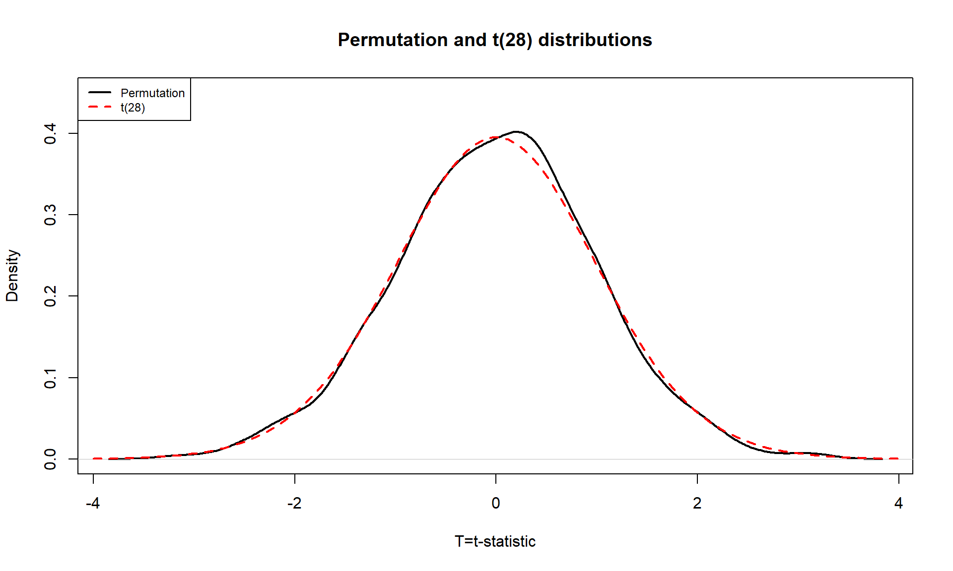
## F-statistic: 4.281 on 1 and 28 DF,  p-value: 0.04789

So the parametric $t$-test gives a p-value of 0.0479 from a test statistic of -2.07. The p-value is very similar to the two permutation results found before. The reason for this similarity is that the permutation distribution looks like a $t$-distribution with 28 degrees of freedom. Figure 2.14 shows how similar the two distributions happened to be here, where the only difference in shape is near the peak of the distributions with a slight difference of the permutation distribution to shift to the right.

Figure 2.14: Plot of permutation and $t$-distribution with $df = 28$. Note the close match in the two distributions, especially in the tails of the distributions where we are obtaining the p-values.

In your previous statistics course, you might have used an applet or a table to find p-values such as what was provided in the previous R output. When not directly provided in the output of a function, R can be used to look up p-values⁴⁴ from named distributions such as the $t$-distribution. In this case, the distribution of the test statistic under the null hypothesis is a $t(28)$ or a $t$ with 28 degrees of freedom. The pt function is used to get p-values from the $t$-distribution in the same manner that pdata could help us to find p-values from the permutation distribution. We need to provide the df = ... and specify the tail of the distribution of interest using the lower.tail option along with the cutoff of interest. If we want the area to the left of -2.07:

pt(-2.069, df = 28, lower.tail = T)

## [1] 0.02394519

And we can double it to get the p-value that was in the output, because the $t$-distribution is symmetric:

2*pt(-2.069, df = 28, lower.tail = T)

## [1] 0.04789038

More generally, we could always make the test statistic positive using the absolute value (abs), find the area to the right of it (lower.tail = F), and then double that for a two-sided test p-value:

2*pt(abs(-2.069), df = 28, lower.tail = F)

## [1] 0.04789038

Permutation distributions do not need to match the named parametric distribution to work correctly, although this happened in the previous example. The parametric approach, the $t$-test, requires certain conditions to be true (or at least not be clearly violated) for the sampling distribution of the statistic to follow the named distribution and provide accurate p-values. The conditions for the $t$-test are:

Independent observations: Each observation obtained is unrelated to all other observations. To assess this, consider whether anything in the data collection might lead to clustered or related observations that are un-related to the differences in the groups. For example, was the same person measured more than once⁴⁵?
Equal variances in the groups (because we used a procedure that assumes equal variances! – there is another procedure that allows you to relax this assumption if needed…). To assess this, compare the standard deviations and variability in the pirate-plots and see if they look noticeably different. Be particularly critical of this assessment if the sample sizes differ greatly between groups.
Normal distributions of the observations in each group. We’ll learn more diagnostics later, but the pirate-plots are a good place to start to help you look for potential skew or outliers. If you find skew and/or outliers, that would suggest a problem with the assumption of normality as normal distributions are symmetric and extreme observations occur very rarely.

For the permutation test, we relax the third condition and replace it with:

Similar distributions for the groups: The permutation approach allows valid inferences as long as the two groups have similar shapes and only possibly differ in their centers. In other words, the distributions need not look normal for the procedure to work well, but they do need to look similar.

In the bicycle overtake study, the independent observation condition is violated because of multiple measurements taken on the same ride. The fact that the same rider was used for all observations is not really a violation of independence here because there was only one subject used. If multiple subjects had been used, then that also could present a violation of the independence assumption. This violation is important to note as the inferences may not be correct due to the violation of this assumption and more sophisticated statistical methods would be needed to complete this analysis correctly. The equal variance condition does not appear to be violated. The standard deviations are 28.4 vs 39.4, so this difference is not “large” according to the rule of thumb noted above (ratio of SDs is about 1.4). There is also little evidence in the pirate-plots to suggest a violation of the normality condition for each of the groups (Figure 2.5). Additionally, the shapes look similar for the two groups so we also could feel comfortable using the permutation approach based on its version of condition (3) above. Note that when assessing assumptions, it is important to never state that assumptions are met – we never know the truth and can only look at the information in the sample to look for evidence of problems with particular conditions. Violations of those conditions suggest a need for either more sophisticated statistical tools⁴⁶ or possibly transformations of the response variable (discussed in Chapter 7).

The permutation approach is resistant to impacts of violations of the normality assumption. It is not resistant to impacts of violations of any of the other assumptions. In fact, it can be quite sensitive to unequal variances as it will detect differences in the variances of the groups instead of differences in the means. Its scope of inference is the same as the parametric approach. It also provides similarly inaccurate conclusions in the presence of non-independent observations as for the parametric approach. In this example, we discover that parametric and permutation approaches provide very similar inferences, but both are subject to concerns related to violations of the independent observations condition. And we haven’t directly addressed the size and direction of the differences, which is addressed in the coming discussion of confidence intervals.

For comparison, we can also explore the original data set of all $n = 1,636$ observations for the two outfits. The estimated difference in the means is -3.003 cm (commute minus casual), the standard error is 1.472, the $t$-statistic is -2.039 and using a $t$-distribution with 1634 $df$, the p-value is 0.0416. The estimated difference in the means is much smaller but the p-value is similar to the results for the sub-sample we analyzed. The SE is much smaller with the large sample size which corresponds to having higher power to detect smaller differences.

lm_all <- lm(Distance ~ Condition, data = ddsub)
summary(lm_all)

## 
## Call:
## lm(formula = Distance ~ Condition, data = ddsub)
## 
## Residuals:
##      Min       1Q   Median       3Q      Max 
## -106.608  -17.608    0.389   16.392  127.389 
## 
## Coefficients:
##                  Estimate Std. Error t value Pr(>|t|)
## (Intercept)       117.611      1.066 110.357   <2e-16
## Conditioncommute   -3.003      1.472  -2.039   0.0416
## 
## Residual standard error: 29.75 on 1634 degrees of freedom
## Multiple R-squared:  0.002539,   Adjusted R-squared:  0.001929 
## F-statistic:  4.16 on 1 and 1634 DF,  p-value: 0.04156

The permutations take a little more computing power with almost two thousand observations to shuffle, but this is manageable on a modern laptop as it only has to be completed once to fill in the distribution of the test statistic under 1,000 shuffles. And the p-value obtained is a close match to the parametric result at 0.045 for the permutation version and 0.042 for the parametric approach. So we would get similar inferences for strength of evidence against the null with either the smaller data set or the full data set but the estimated size of the differences is quite a bit different. It is important to note that other random samples from the larger data set would give different p-values and this one happened to match the larger set more closely than one might expect in general.

Tobs <- summary(lm_all)$coef[2,3]
Tobs

## [1] -2.039491

B <- 1000
set.seed(406)
Tstar <- matrix(NA, nrow = B)
for (b in (1:B)){
  lmP <- lm(Distance ~ shuffle(Condition), data = ddsub)
  Tstar[b] <- summary(lmP)$coef[2,3]
}
pdata(abs(Tstar), abs(Tobs), lower.tail = F)

## [1] 0.045

Figure 2.15: Permutation distribution of the $t$-statistic for $n = 1,636$ overtake data set.