2.3: Models, hypotheses, and permutations for the two sample mean situation

Last updated
Save as PDF

Page ID: 33216

\( \newcommand{\vecs}[1]{\overset { \scriptstyle \rightharpoonup} {\mathbf{#1}} } \) \( \newcommand{\vecd}[1]{\overset{-\!-\!\rightharpoonup}{\vphantom{a}\smash {#1}}} \)\(\newcommand{\id}{\mathrm{id}}\) \( \newcommand{\Span}{\mathrm{span}}\) \( \newcommand{\kernel}{\mathrm{null}\,}\) \( \newcommand{\range}{\mathrm{range}\,}\) \( \newcommand{\RealPart}{\mathrm{Re}}\) \( \newcommand{\ImaginaryPart}{\mathrm{Im}}\) \( \newcommand{\Argument}{\mathrm{Arg}}\) \( \newcommand{\norm}[1]{\| #1 \|}\) \( \newcommand{\inner}[2]{\langle #1, #2 \rangle}\) \( \newcommand{\Span}{\mathrm{span}}\) \(\newcommand{\id}{\mathrm{id}}\) \( \newcommand{\Span}{\mathrm{span}}\) \( \newcommand{\kernel}{\mathrm{null}\,}\) \( \newcommand{\range}{\mathrm{range}\,}\) \( \newcommand{\RealPart}{\mathrm{Re}}\) \( \newcommand{\ImaginaryPart}{\mathrm{Im}}\) \( \newcommand{\Argument}{\mathrm{Arg}}\) \( \newcommand{\norm}[1]{\| #1 \|}\) \( \newcommand{\inner}[2]{\langle #1, #2 \rangle}\) \( \newcommand{\Span}{\mathrm{span}}\)\(\newcommand{\AA}{\unicode[.8,0]{x212B}}\)

There appears to be some evidence that the casual clothing group is getting higher average overtake distances than the commute group of observations, but we want to try to make sure that the difference is real – to assess evidence against the assumption that the means are the same “in the population” and possibly decide that this is not a reasonable assumption. First, a null hypothesis²⁷ which defines a null model²⁸ needs to be determined in terms of parameters (the true values in the population). The research question should help you determine the form of the hypotheses for the assumed population. In the two independent sample mean problem, the interest is in testing a null hypothesis of \(H_0: \mu_1 = \mu_2\) versus the alternative hypothesis of \(H_A: \mu_1 \ne \mu_2\), where \(\mu_1\) is the parameter for the true mean of the first group and \(\mu_2\) is the parameter for the true mean of the second group. The alternative hypothesis involves assuming a statistical model for the \(i^{th}\ (i = 1,\ldots,n_j)\) response from the \(j^{th}\ (j = 1,2)\) group, \(\boldsymbol{y}_{ij}\), that involves modeling it as \(y_{ij} = \mu_j + \varepsilon_{ij}\), where we assume that \(\varepsilon_{ij} \sim N(0,\sigma^2)\). For the moment, focus on the models that either assume the means are the same (null) or different (alternative), which imply:

Null Model: \(y_{ij} = \mu + \varepsilon_{ij}\) There is no difference in true means for the two groups.
Alternative Model: \(y_{ij} = \mu_j + \varepsilon_{ij}\) There is a difference in true means for the two groups.

Suppose we are considering the alternative model for the 4^th observation (\(i = 4\)) from the second group (\(j = 2\)), then the model for this observation is \(y_{42} = \mu_2 +\varepsilon_{42}\), that defines the response as coming from the true mean for the second group plus a random error term for that observation, \(\varepsilon_{42}\). For, say, the 5^th observation from the first group (\(j = 1\)), the model is \(y_{51} = \mu_1 +\varepsilon_{51}\). If we were working with the null model, the mean is always the same (\(\mu\)) – the group specified does not change the mean we use for that observation, so the model for \(y_{42}\) would be \(\mu +\varepsilon_{42}\).

It can be helpful to think about the null and alternative models graphically. By assuming the null hypothesis is true (means are equal) and that the random errors around the mean follow a normal distribution, we assume that the truth is as displayed in the left panel of Figure 2.6 – two normal distributions with the same mean and variability. The alternative model allows the two groups to potentially have different means, such as those displayed in the right panel of Figure 2.6 where the second group has a larger mean. Note that in this scenario, we assume that the observations all came from the same distribution except that they had different means. Depending on the statistical procedure we are using, we basically are going to assume that the observations (\(y_{ij}\)) either were generated as samples from the null or alternative model. You can imagine drawing observations at random from the pictured distributions. For hypothesis testing, the null model is assumed to be true and then the unusualness of the actual result is assessed relative to that assumption. In hypothesis testing, we have to decide if we have enough evidence to reject the assumption that the null model (or hypothesis) is true. If we think that we have sufficient evidence to conclude that the null hypothesis is wrong, then we would conclude that the other model considered (the alternative model) is more reasonable. The researchers obviously would have hoped to encounter some sort of noticeable difference in the distances for the different outfits and have been able to find enough evidence to against the null model where the groups “look the same” to be able to conclude that they differ.

Figure 2.6: Illustration of the assumed situations under the null (left) and a single possibility that could occur if the alternative were true (right) and the true means were different. There are an infinite number of ways to make a plot like the right panel that satisfies the alternative hypothesis.

In statistical inference, null hypotheses (and their implied models) are set up as “straw men” with every interest in rejecting them even though we assume they are true to be able to assess the evidence \(\underline{\text{against them}}\). Consider the original study design here, the outfits were randomly assigned to the rides. If the null hypothesis were true, then we would have no difference in the population means of the groups. And this would apply if we had done a different random assignment of the outfits. So let’s try this: assume that the null hypothesis is true and randomly re-assign the treatments (outfits) to the observations that were obtained. In other words, keep the Distance results the same and shuffle the group labels randomly. The technical term for this is doing a permutation (a random shuffling of a grouping²⁹ variable relative to the observed responses). If the null is true and the means in the two groups are the same, then we should be able to re-shuffle the groups to the observed Distance values and get results similar to those we actually observed. If the null is false and the means are really different in the two groups, then what we observed should differ from what we get under other random permutations and the differences between the two groups should be more noticeable in the observed data set than in (most) of the shuffled data sets. It helps to see an example of a permutation of the labels to understand what this means here.

The data set we are working with is a little on the large size, especially to explore individual observations. So for the moment we are going to work with a random sample of 30 of the \(n = 1,636\) observations in ddsub, fifteen from each group, that are generated using the sample function. To do this³⁰, we will use the sample function twice – once to sample from the subsetted commute observations (creating the s1 data set) and once to sample from the casual ones (creating s2). A new function for us, called rbind, is used to bind the rows together — much like pasting a chunk of rows below another chunk in a spreadsheet program. This operation only works if the columns all have the same names and meanings both for rbind and in a spreadsheet. Together this code creates the dsample data set that we will analyze below and compare to results from the full data set. The sample means are now 135.8 and 109.87 cm for casual and commute groups, respectively, and so the difference in the sample means has increased in magnitude to -25.93 cm (commute - casual). This difference would vary based on the different random samples from the larger data set, but for the moment, pretend this was the entire data set that the researchers had collected and that we want to try to assess how unusual our sample difference was from what we might expect, if the null hypothesis that the true means are the same in these two groups was true.

set.seed(9432)
s1 <- sample(ddsub %>% filter(Condition %in% "commute"), size = 15)
s2 <- sample(ddsub %>% filter(Condition %in% "casual"), size = 15)
dsample <- rbind(s1, s2)
mean(Distance ~ Condition, data = dsample)

##   casual  commute 
## 135.8000 109.8667

In order to assess evidence against the null hypothesis of no difference, we want to permute the group labels versus the observations. In the mosaic package, the shuffle function allows us to easily perform a permutation³¹. One permutation of the treatment labels is provided in the PermutedCondition variable below. Note that the Distances are held in the same place while the group labels are shuffled.

Perm1 <- dsample %>% 
  select(Distance, Condition) %>% 
  mutate(PermutedCondition = shuffle(Condition))
# To force the tibble to print out all rows in data set -- not used often
data.frame(Perm1)

##    Distance Condition PermutedCondition
## 1       168   commute           commute
## 2       137   commute           commute
## 3        80   commute            casual
## 4       107   commute           commute
## 5       104   commute            casual
## 6        60   commute            casual
## 7        88   commute           commute
## 8       126   commute           commute
## 9       115   commute            casual
## 10      120   commute            casual
## 11      146   commute           commute
## 12      113   commute            casual
## 13       89   commute           commute
## 14       77   commute           commute
## 15      118   commute            casual
## 16      148    casual            casual
## 17      114    casual            casual
## 18      124    casual           commute
## 19      115    casual            casual
## 20      102    casual            casual
## 21       77    casual            casual
## 22       72    casual           commute
## 23      193    casual           commute
## 24      111    casual           commute
## 25      161    casual            casual
## 26      208    casual           commute
## 27      179    casual            casual
## 28      143    casual           commute
## 29      144    casual           commute
## 30      146    casual            casual

If you count up the number of subjects in each group by counting the number of times each label (commute, casual) occurs, it is the same in both the Condition and PermutedCondition columns (15 each). Permutations involve randomly re-ordering the values of a variable – here the Condition group labels – without changing the content of the variable. This result can also be generated using what is called sampling without replacement: sequentially select \(n\) labels from the original variable (Condition), removing each observed label and making sure that each of the original Condition labels is selected once and only once. The new, randomly selected order of selected labels provides the permuted labels. Stepping through the process helps to understand how it works: after the initial random sample of one label, there would \(n - 1\) choices possible; on the \(n^{th}\) selection, there would only be one label remaining to select. This makes sure that all original labels are re-used but that the order is random. Sampling without replacement is like picking names out of a hat, one-at-a-time, and not putting the names back in after they are selected. It is an exhaustive process for all the original observations. Sampling with replacement, in contrast, involves sampling from the specified list with each observation having an equal chance of selection for each sampled observation – in other words, observations can be selected more than once. This is like picking \(n\) names out of a hat that contains \(n\) names, except that every time a name is selected, it goes back into the hat – we’ll use this technique in Section 2.9 to do what is called bootstrapping. Both sampling mechanisms can be used to generate inferences but each has particular situations where they are most useful. For hypothesis testing, we will use permutations (sampling without replacement) as its mechanism most closely matches the null hypotheses we will be testing.

The comparison of the pirate-plots between the real \(n = 30\) data set and permuted version is what is really interesting (Figure 2.7). The original difference in the sample means of the two groups was -25.93 cm (commute - casual). The sample means are the statistics that estimate the parameters for the true means of the two groups and the difference in the sample means is a way to create a single number that tracks a quantity directly related to the difference between the null and alternative models. In the permuted data set, the difference in the means is 12.07 cm in the opposite direction (the commute group had a higher mean than casual in the permuted data).

mean(Distance ~ PermutedCondition, data = Perm1)

##   casual  commute 
## 116.8000 128.8667

diffmean(Distance ~ PermutedCondition, data = Perm1)

## diffmean 
## 12.06667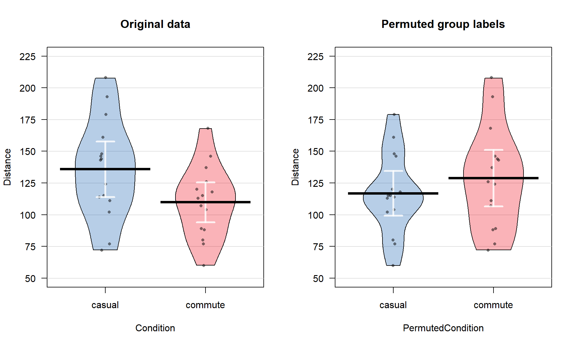

Figure 2.7: Pirate-plots of Distance responses versus actual treatment groups and permuted groups. Note how the responses are the same but that they are shuffled between the two groups differently in the permuted data set. With the smaller sample size, the 95% confidence intervals for each of the means are more clearly visible than with the original large data set.

The diffmean function is a simple way to get the differences in the means, but we can also start to learn about using the lm function – that will be used for every chapter except for Chapter 5. The lm stands for linear model and, as we will see moving forward, encompasses a wide array of different models and scenarios. The ability to estimate the difference in the mean of two groups is among its simplest uses.³² Notationally, it is very similar to other functions we have considered, lm(y ~ x, data = ...) where y is the response variable and x is the explanatory variable. Here that is lm(Distance ~ Condition, data = dsample) with Condition defined as a factor variable. With linear models, we will need to interrogate them to obtain a variety of useful information and our first “interrogation” function is usually the summary function. To use it, it is best to have stored the model into an object, something like lm1, and then we can apply the summary() function to the stored model object to get a suite of output:

lm1 <- lm(Distance ~ Condition, data = dsample)
summary(lm1)

## 
## Call:
## lm(formula = Distance ~ Condition, data = dsample)
## 
## Residuals:
##     Min      1Q  Median      3Q     Max 
## -63.800 -21.850   4.133  15.150  72.200 
## 
## Coefficients:
##                  Estimate Std. Error t value Pr(>|t|)
## (Intercept)       135.800      8.863  15.322 3.83e-15
## Conditioncommute  -25.933     12.534  -2.069   0.0479
## 
## Residual standard error: 34.33 on 28 degrees of freedom
## Multiple R-squared:  0.1326, Adjusted R-squared:  0.1016 
## F-statistic: 4.281 on 1 and 28 DF,  p-value: 0.04789

This output is explored more in Chapter 3, but for the moment, focus on the row labeled as Conditioncommute in the middle of the output. In the first (Estimate) column, there is -25.933. This is a number we saw before – it is the difference in the sample means between commute and casual (commute - casual). When lm denotes a category in the row of the output (here commute), it is trying to indicate that the information to follow relates to the difference between this category and a baseline or reference category (here casual). The first ((Intercept)) row also contains a number we have seen before: -135.8 is the sample mean for the casual group. So the lm is generating a coefficient for the mean of one of the groups and another as the difference in the two groups³³. In developing a test to assess evidence against the null hypothesis, we will focus on the difference in the sample means. So we want to be able to extract that number from this large suite of information. It ends up that we can apply the coef function to lm models and then access that second coefficient using the bracket notation. Specifically:

coef(lm1)[2]

## Conditioncommute 
##        -25.93333

This is the same result as using the diffmean function, so either could be used here. The estimated difference in the sample means in the permuted data set of 12.07 cm is available with:

lmP <- lm(Distance ~ PermutedCondition, data = Perm1)
coef(lmP)[2]

## PermutedConditioncommute 
##                 12.06667

Comparing the pirate-plots and the estimated difference in the sample means suggests that the observed difference was larger than what we got when we did a single permutation. Conceptually, permuting observations between group labels is consistent with the null hypothesis – this is a technique to generate results that we might have gotten if the null hypothesis were true since the true models for the responses are the same in the two groups if the null is true. We just need to repeat the permutation process many times and track how unusual our observed result is relative to this distribution of potential responses if the null were true. If the observed differences are unusual relative to the results under permutations, then there is evidence against the null hypothesis, and we can conclude, in the direction of the alternative hypothesis, that the true means differ. If the observed differences are similar to (or at least not unusual relative to) what we get under random shuffling under the null model, we would have a tough time concluding that there is any real difference between the groups based on our observed data set. This is formalized using the p-value as a measure of the strength of evidence against the null hypothesis and how we use it.