3.6: Polynomial Functions
- Page ID
- 34413
\( \newcommand{\vecs}[1]{\overset { \scriptstyle \rightharpoonup} {\mathbf{#1}} } \)
\( \newcommand{\vecd}[1]{\overset{-\!-\!\rightharpoonup}{\vphantom{a}\smash {#1}}} \)
\( \newcommand{\dsum}{\displaystyle\sum\limits} \)
\( \newcommand{\dint}{\displaystyle\int\limits} \)
\( \newcommand{\dlim}{\displaystyle\lim\limits} \)
\( \newcommand{\id}{\mathrm{id}}\) \( \newcommand{\Span}{\mathrm{span}}\)
( \newcommand{\kernel}{\mathrm{null}\,}\) \( \newcommand{\range}{\mathrm{range}\,}\)
\( \newcommand{\RealPart}{\mathrm{Re}}\) \( \newcommand{\ImaginaryPart}{\mathrm{Im}}\)
\( \newcommand{\Argument}{\mathrm{Arg}}\) \( \newcommand{\norm}[1]{\| #1 \|}\)
\( \newcommand{\inner}[2]{\langle #1, #2 \rangle}\)
\( \newcommand{\Span}{\mathrm{span}}\)
\( \newcommand{\id}{\mathrm{id}}\)
\( \newcommand{\Span}{\mathrm{span}}\)
\( \newcommand{\kernel}{\mathrm{null}\,}\)
\( \newcommand{\range}{\mathrm{range}\,}\)
\( \newcommand{\RealPart}{\mathrm{Re}}\)
\( \newcommand{\ImaginaryPart}{\mathrm{Im}}\)
\( \newcommand{\Argument}{\mathrm{Arg}}\)
\( \newcommand{\norm}[1]{\| #1 \|}\)
\( \newcommand{\inner}[2]{\langle #1, #2 \rangle}\)
\( \newcommand{\Span}{\mathrm{span}}\) \( \newcommand{\AA}{\unicode[.8,0]{x212B}}\)
\( \newcommand{\vectorA}[1]{\vec{#1}} % arrow\)
\( \newcommand{\vectorAt}[1]{\vec{\text{#1}}} % arrow\)
\( \newcommand{\vectorB}[1]{\overset { \scriptstyle \rightharpoonup} {\mathbf{#1}} } \)
\( \newcommand{\vectorC}[1]{\textbf{#1}} \)
\( \newcommand{\vectorD}[1]{\overrightarrow{#1}} \)
\( \newcommand{\vectorDt}[1]{\overrightarrow{\text{#1}}} \)
\( \newcommand{\vectE}[1]{\overset{-\!-\!\rightharpoonup}{\vphantom{a}\smash{\mathbf {#1}}}} \)
\( \newcommand{\vecs}[1]{\overset { \scriptstyle \rightharpoonup} {\mathbf{#1}} } \)
\(\newcommand{\longvect}{\overrightarrow}\)
\( \newcommand{\vecd}[1]{\overset{-\!-\!\rightharpoonup}{\vphantom{a}\smash {#1}}} \)
\(\newcommand{\avec}{\mathbf a}\) \(\newcommand{\bvec}{\mathbf b}\) \(\newcommand{\cvec}{\mathbf c}\) \(\newcommand{\dvec}{\mathbf d}\) \(\newcommand{\dtil}{\widetilde{\mathbf d}}\) \(\newcommand{\evec}{\mathbf e}\) \(\newcommand{\fvec}{\mathbf f}\) \(\newcommand{\nvec}{\mathbf n}\) \(\newcommand{\pvec}{\mathbf p}\) \(\newcommand{\qvec}{\mathbf q}\) \(\newcommand{\svec}{\mathbf s}\) \(\newcommand{\tvec}{\mathbf t}\) \(\newcommand{\uvec}{\mathbf u}\) \(\newcommand{\vvec}{\mathbf v}\) \(\newcommand{\wvec}{\mathbf w}\) \(\newcommand{\xvec}{\mathbf x}\) \(\newcommand{\yvec}{\mathbf y}\) \(\newcommand{\zvec}{\mathbf z}\) \(\newcommand{\rvec}{\mathbf r}\) \(\newcommand{\mvec}{\mathbf m}\) \(\newcommand{\zerovec}{\mathbf 0}\) \(\newcommand{\onevec}{\mathbf 1}\) \(\newcommand{\real}{\mathbb R}\) \(\newcommand{\twovec}[2]{\left[\begin{array}{r}#1 \\ #2 \end{array}\right]}\) \(\newcommand{\ctwovec}[2]{\left[\begin{array}{c}#1 \\ #2 \end{array}\right]}\) \(\newcommand{\threevec}[3]{\left[\begin{array}{r}#1 \\ #2 \\ #3 \end{array}\right]}\) \(\newcommand{\cthreevec}[3]{\left[\begin{array}{c}#1 \\ #2 \\ #3 \end{array}\right]}\) \(\newcommand{\fourvec}[4]{\left[\begin{array}{r}#1 \\ #2 \\ #3 \\ #4 \end{array}\right]}\) \(\newcommand{\cfourvec}[4]{\left[\begin{array}{c}#1 \\ #2 \\ #3 \\ #4 \end{array}\right]}\) \(\newcommand{\fivevec}[5]{\left[\begin{array}{r}#1 \\ #2 \\ #3 \\ #4 \\ #5 \\ \end{array}\right]}\) \(\newcommand{\cfivevec}[5]{\left[\begin{array}{c}#1 \\ #2 \\ #3 \\ #4 \\ #5 \\ \end{array}\right]}\) \(\newcommand{\mattwo}[4]{\left[\begin{array}{rr}#1 \amp #2 \\ #3 \amp #4 \\ \end{array}\right]}\) \(\newcommand{\laspan}[1]{\text{Span}\{#1\}}\) \(\newcommand{\bcal}{\cal B}\) \(\newcommand{\ccal}{\cal C}\) \(\newcommand{\scal}{\cal S}\) \(\newcommand{\wcal}{\cal W}\) \(\newcommand{\ecal}{\cal E}\) \(\newcommand{\coords}[2]{\left\{#1\right\}_{#2}}\) \(\newcommand{\gray}[1]{\color{gray}{#1}}\) \(\newcommand{\lgray}[1]{\color{lightgray}{#1}}\) \(\newcommand{\rank}{\operatorname{rank}}\) \(\newcommand{\row}{\text{Row}}\) \(\newcommand{\col}{\text{Col}}\) \(\renewcommand{\row}{\text{Row}}\) \(\newcommand{\nul}{\text{Nul}}\) \(\newcommand{\var}{\text{Var}}\) \(\newcommand{\corr}{\text{corr}}\) \(\newcommand{\len}[1]{\left|#1\right|}\) \(\newcommand{\bbar}{\overline{\bvec}}\) \(\newcommand{\bhat}{\widehat{\bvec}}\) \(\newcommand{\bperp}{\bvec^\perp}\) \(\newcommand{\xhat}{\widehat{\xvec}}\) \(\newcommand{\vhat}{\widehat{\vvec}}\) \(\newcommand{\uhat}{\widehat{\uvec}}\) \(\newcommand{\what}{\widehat{\wvec}}\) \(\newcommand{\Sighat}{\widehat{\Sigma}}\) \(\newcommand{\lt}{<}\) \(\newcommand{\gt}{>}\) \(\newcommand{\amp}{&}\) \(\definecolor{fillinmathshade}{gray}{0.9}\)A Polynomial Function is a function that can be written in the general form:
\(f(x) = a_n x^n + a_{n−1} x^{n−1 }+ ... + a_1x + a_0\)
for \(n\) a non-negative integer, called the degree of the polynomial. The coefficients \(a_0\), \(a_1\), \(\ldots\), an are real numbers with leading coefficient an \(a_n \neq 0\). The domain of a Polynomial Function is \((−\infty , \infty )\). The graph of a polynomial function of degree \(n\) can intersect the x-axis at most \(n\) times. These are the roots of the polynomial function.
There are no examples or homework in this section.
Quadratic Functions
\(f(x) = ax^2 + bx + c\) where \(a\neq 0\)
is a Quadratic Function in standard form, and its graph is a parabola. When the leading coefficient, \(a\), is positive, the graph of the Quadratic Function opens upward. When the leading coefficient, \(a\), is negative, the graph of the Quadratic Function opens downward.
Sketch a graph of \(f(x) = −x^2 + 5x + 3\) in a rectangular coordinate system. Find the vertex, the x-intercept(s) and the y-intercept algebraically.
Solution
Find the vertex by calculating \(\left(\dfrac{-b}{2 a}, f\left(\dfrac{-b}{2 a}\right)\right)\) with \(a = −1\), \(b = 5\) and \(c = 3\).
\(\begin{aligned}
\left(\dfrac{-b}{2 a}, f\left(\dfrac{-b}{2 a}\right)\right)&=&& \text { Find the vertex of the parabola }\\
\dfrac{-5}{2(-1)}&=\\
\dfrac{5}{2}&=2.5 &&\text { Simplify }\\
\dfrac{-5}{2(-1)}&=2.5\\
f(2.5)&=-(2.5)^{2}+5(2.5)+3=9.25=&& f\left(\dfrac{-b}{2 a}\right)=9.25\\ \left(\dfrac{-b}{2 a}, f\left(\dfrac{-b}{2 a}\right)\right)&=(2.5,9.25) && \text { Vertex of the parabola }
\end{aligned}\)
To find the intercepts:
\(\begin{aligned} 0&=-x^{2}+5 x+3 && \text{x-intercept, set } f(x)=0 \\ 0&=-x^{2}+5 x+3 && \text{Use the Quadratic Formula to solve this equation (it can't be factored). Let } a=-1, b=5, c=3 \\ x&=\dfrac{-5 \pm \sqrt{(5)^{2}-4(-1)(3)}}{2(-1)} &&\text{Quadratic Formula
} \\ x&=\dfrac{-5 \pm \sqrt{37}}{-2} && \text{Simplify} \\
x&=-0.54 \text{ or } x=5.54 && \text{This quadratic function has two roots (x-intercepts).} \\ f(0)&=-0^{2}+5(0)+3 && \text{y-intercept, set } x=0 \\ f(0)&=3 && \text{y-intercept} \end{aligned}\)
Graph the four ordered pairs, and calculate more ordered pairs if needed: \((2.5, 9.25)\), \((−.54, 0)\), \((5.54, 0)\), \((0, 3)\).
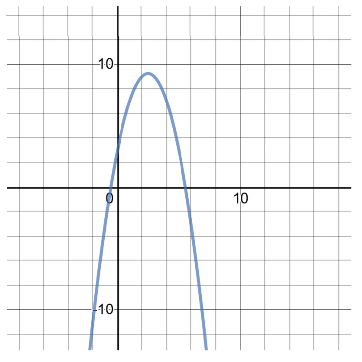 Figure 4.6.1
- \(f(x) = 2x ^2 − 5x − 5\)
- \(f(x) = 0.5x ^2 − 6x + 21\)
- \(f(x) = −4x ^2 − 8x − 3\)
- \(f(x) = −4x^ 2 + 16x − 15\)
- \(f(x) = x^ 2 − 8x + 12\)
- \(f(x) = −7x^ 2 + 100x − 10\)
Cubic and Higher Order Functions
A Cubic Function is a third-degree polynomial function that can be written in the general form:
\(f(x) = a_3x^ 3 + a_2x^2 + a_1x + a_0\)
with 3 as the degree of the cubic function. The coefficients \(a_0\), \(a_1\), \(a_2\), \(a_3\) are real numbers with leading coefficient \(a_3 \neq 0\). The domain of a cubic function is \((−\infty , \infty )\).
Factor if possible and graph the function by creating a table of solutions:
\(f(x) = x^3 − 4x^2 + 6x − 1\)
Solution
This polynomial is of degree 3, and is difficult to factor. Create a table of solutions to graph.
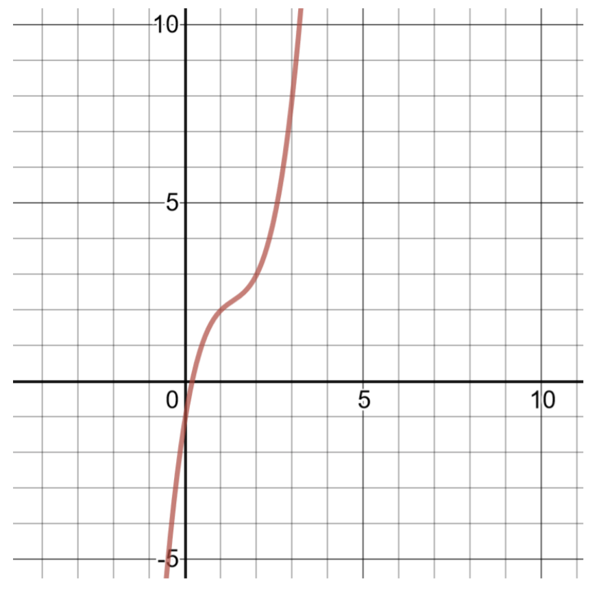 Figure 4.6.2
| Table of Solutions for \(f(x) = x^3 − 4x^2 + 6x − 1\) | |
| \(x\) | \(f(x)\) |
| -2 | \(f(−2) = (−2)^3 − 4(−2)^2 + 6(−2) − 1 = −37\) |
| -1 | \(f(−1) = (−1)^3 − 4(−1)^2 + 6(−1) − 1 = −12\) |
| 0 | \(f(0) = (0)^3 − 4(0)^2 + 6(0) − 1 = −1\) |
| 1 | \(f(1) = (1)^3 − 4(1)^2 + 6(1) − 1 = 2\) |
| 2 | \(f(2) = (2)^3 − 4(2)^2 + 6(2) − 1 = 3\) |
Factor if possible and graph the function by creating a table of solutions:
\(g(x)=x^4-16\)
Solution
This polynomial is of degree 4, and because it is a difference of squares, it can be factored into a product of binomials to find the zeroes of the polynomial. Create a table of solutions to graph.
\(\begin{aligned} g(x)&=\left(x^{2}-4\right)\left(x^{2}+4\right) && \text{Factoring into the sum and difference of binomials.} \\ g(x)&=(x-2)(x+2)\left(x^{2}+4\right) && \text{Further factoring. Set each binomial equal to zero to find the real number zeroes of the polynomial.} \\ x-2&=0, x=2 && \text{The first real number zero of the polynomial, }(2,0) \\ x+2&=0, x=-2 &&\text{The second real number zero of the polynomial, } (2,0) \\ x^{2}+4&=0, x^{2}=-4 && \text{The third binomial factor does not produce real number zeroes, } \\ & &&\text{because no number squared can result in a negative value.} \end{aligned}\)
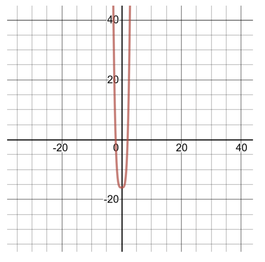 Figure 4.6.3
| Table of Solutions for \(g(x)=x^4-16\) | |
| \(x\) | \(g(x)\) |
| -2 | \(g(−2) = (−2)^4 − 16 = 16 − 16 = 0\) |
| -1 | \(g(−1) = (−1)^4 − 16 = 1 − 16 = −15\) |
| 0 | \(g(0) = (0)^4 − 16 = 0 − 16 = −16\) |
| 1 | \(g(1) = g(1) = (1)^4 − 16 = 1 − 16 = −15\) |
| 2 | \(g(2) = g(2) = (2)^4 − 16 = 16 − 16 = 0\) |
Factor if possible and graph the function by creating a table of solutions:
\(f(x) = x ^6 − 5x ^2 + 3\)
Solution
This polynomial is of degree 6, and is difficult to factor. Create a table of solutions to graph.
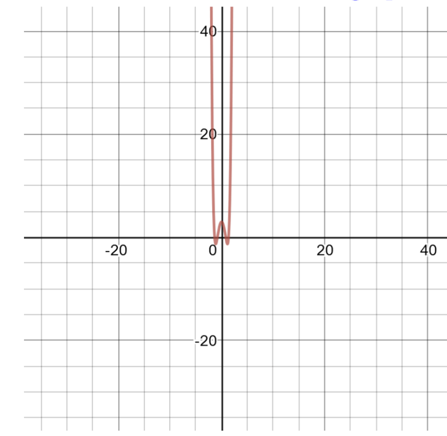 Figure 4.6.4
| Table of Solutions for \(f(x) = x ^6 − 5x ^2 + 3\) | |
| \(x\) | \(f(x)\) |
| -2 | \(f(−2) = (−2)^6 − 5(−2)^2 + 3 = 47\) |
| -1 | \(f(−1) = (−1)^6 − 5(−1)^2 + 3 = −1\) |
| 0 | \(f(0) = (0)^6 − 5(0)^2 + 3 = 3\) |
| 1 | \(f(1) = (1)^6 − 5(1)^2 + 3 = −1\) |
| 2 | \(f(2) = (2)^6 − 5(2)^2 + 3 = 47\) |
- \(f(x) = x^3 − 27\)
- \(g(x) = 81x ^4 − 16\)
- \(h(x) = 2x ^5 − 4x ^2 − 6x + 3\)
- \(f(x) = 5x ^6 − 6x ^4 + 5\)
Rational Functions
A rational function is a function that can be written as a quotient of polynomials.
\(f(x) = \dfrac{P (x) }{Q(x) }\), \(Q(x) \neq 0\)
where \(P(x)\) and \(Q(x)\) are polynomials in one variable \(x\). The domain is the set of all real numbers such that \(Q(x) \neq 0\).
For the function, \(f(x) = \dfrac{9 }{x − 3}\) :
- Graph the function
- Evaluate the function for \(x = 0\) and \(x = 2\)
Solution
Pay attention to the domain of this function. Division by zero is undefined, so the number(s) that will make the denominator 0 must be excluded from the domain.
In this problem, \(x − 3\) is in the denominator of the function. Set \(x − 3 = 0\) and solve for \(x\). If \(x = 3\) the division is undefined, so exclude the number 3 from the domain of the function. Think of it as always starting with all real numbers \((−\infty , \infty )\) and then removing the values that will cause undefined division.
The domain of this function is \((−\infty , 3) \cup (3, \infty )\).
Rational functions will often have asymptotes, a line that continually approaches a given curve but does not meet it at any finite distance. You will learn about asymptotes in the Curve Sketching section of Math 162.
The graph of this function can be found by making a table of solutions:
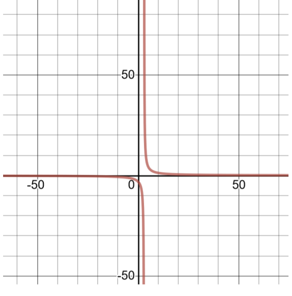 Figure 4.6.5
| Table of Solutions for \(f(x) = \dfrac{9 }{x − 3}\) | Domain: \((−\infty , 3) \cup (3, \infty )\) |
| \(x\) | \(f(x)\) |
| -4 | \(-\dfrac{9}{7}\) |
| -3 | \(-\dfrac{3}{2}\) |
| -2 | \(-\dfrac{9}{5}\) |
| -1 | \(-\dfrac{9}{4}\) |
| 0 | \(-3\) |
| 1 | \(-\dfrac{9}{2}\) |
| 2 | \(-9\) |
For the function, \(f(x) = \dfrac{100x}{ x^2 − 3x − 4}\)
- Graph the function
- Evaluate the function for \(x = −1\) and \(x = 3\)
Solution
Pay attention to the domain of this function. Division by zero is undefined, so the number(s) that will make the denominator 0 must be excluded from the domain.
In this problem, \(x^2 − 3x − 4\) is in the denominator of the function. Factor the quadratic expression to get \((x − 4)(x + 1)\) and set each factor equal to zero and solve for \(x\): \(x − 4 = 0\), so \(x = 4\); \(x + 1 = 0\), so \(x = −1\). If \(x = 4\) or \(x = −1\), the division is undefined, so exclude the numbers 4 and −1 from the domain of the function. Think of it as always starting with all real numbers \((−\infty , \infty )\) and then removing the values that will result in undefined division.
The domain of this function is \((−\infty , −1) \cup (−1, 4) \cup (4, \infty )\). The graph of this function can be found by making a table of solutions:
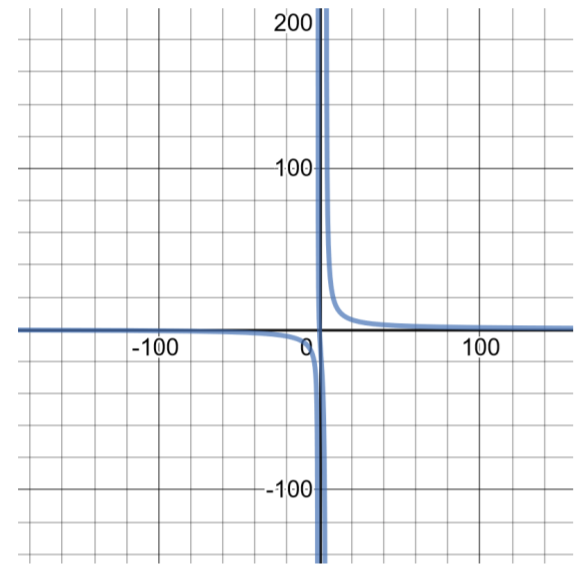 Figure 4.6.6
| Table of Solutions for \(f(x) = \dfrac{100x}{ x^2 − 3x − 4}\) | Domain: \((−\infty , −1) \cup (−1, 4) \cup (4, \infty )\) |
| \(x\) | \(f(x)\) |
| -4 | −16.667 |
| -3 | −21.429 |
| -2 | −33.333 |
| -1 | undefined |
| 0 | 0 |
| 1 | −16.667 |
| 2 | −33.333 |
| 3 | -75 |
| 4 | undefined |
- \(f(x) = \dfrac{3x + 6 }{x − 1}\)
- \(f(x) = \dfrac{9 }{x^2 − 9}\)
- \(f(x) = \dfrac{x^ 2 − 4 }{x^2 − 4x}\)


