13.2: Sign Test

Last updated
Save as PDF

Page ID: 24081

$ \newcommand{\vecs}[1]{\overset { \scriptstyle \rightharpoonup} {\mathbf{#1}} } $ $ \newcommand{\vecd}[1]{\overset{-\!-\!\rightharpoonup}{\vphantom{a}\smash {#1}}} $$\newcommand{\id}{\mathrm{id}}$ $ \newcommand{\Span}{\mathrm{span}}$ $ \newcommand{\kernel}{\mathrm{null}\,}$ $ \newcommand{\range}{\mathrm{range}\,}$ $ \newcommand{\RealPart}{\mathrm{Re}}$ $ \newcommand{\ImaginaryPart}{\mathrm{Im}}$ $ \newcommand{\Argument}{\mathrm{Arg}}$ $ \newcommand{\norm}[1]{\| #1 \|}$ $ \newcommand{\inner}[2]{\langle #1, #2 \rangle}$ $ \newcommand{\Span}{\mathrm{span}}$ $\newcommand{\id}{\mathrm{id}}$ $ \newcommand{\Span}{\mathrm{span}}$ $ \newcommand{\kernel}{\mathrm{null}\,}$ $ \newcommand{\range}{\mathrm{range}\,}$ $ \newcommand{\RealPart}{\mathrm{Re}}$ $ \newcommand{\ImaginaryPart}{\mathrm{Im}}$ $ \newcommand{\Argument}{\mathrm{Arg}}$ $ \newcommand{\norm}[1]{\| #1 \|}$ $ \newcommand{\inner}[2]{\langle #1, #2 \rangle}$ $ \newcommand{\Span}{\mathrm{span}}$$\newcommand{\AA}{\unicode[.8,0]{x212B}}$

The sign test can be used for both one sample or for two dependent groups. The sign test uses a Binomial Distribution and looks at the probability of a success as 50%. The median is the 50th percentile, so many times we will state our null hypothesis as the median is equal to a certain value. However, sometimes we will state the hypothesis in terms of a proportion.

Two-Tailed Test	Right-Tailed Test	Left-Tailed Test
$H_{0}:$ Median $= \text{MD}_{0}$ $H_{1}:$ Median $\neq \text{MD}_{0}$	$H_{0}:$ Median $= \text{MD}_{0}$ $H_{1}:$ Median $> \text{MD}_{0}$	$H_{0}:$ Median $= \text{MD}_{0}$ $H_{1}:$ Median $< \text{MD}_{0}$

$\text{MD}_{0}$ is a placeholder for the number for the hypothesized median.

The Sign Test Procedure

For the single-sample test, compare each value with the conjectured median. If a data value is larger than the hypothesized median, replace the value with a positive sign. If a data value is smaller than the hypothesized median, replace the value with a negative sign. If the data value equals the hypothesized median, replace the value with a 0.

The sample size is the number of plus and minus signs added together (do not include data values that tie with the median). For the paired-sample sign test, subtract the group 2 values from the group 1 values and indicate the difference with a positive or negative sign, or 0 (if they tie) and $n$ = total number of positive and negative signs (do not include differences of zero).

Use the binomial distribution to find the p-value using technology.

For a two-tailed test, the test statistic, $x$, is the smaller of the plus or minus signs. If $x$ is the test statistic, the p-value for a two-tailed test is the $2 \cdot \text{P} (X \leq x)$.
For a right-tailed test, the test statistic, $x$, is the number of plus signs. For a left-tailed test, the test statistic, $x$, is the number of minus signs. The p-value for a one-tailed test is the $\text{P} (X \geq x)$.

The sign test is an alternative to the one sample t-test when you have a small sample size, but the population is not normally distributed. The sign test is also an alternative to the paired sample t-test when you have a small sample size and the difference in the pairs is not normally distributed. The sign test does not detect the magnitude of the difference between the hypothesized value and is not as efficient as the t-test.

A student tells her parents that the median rental rate for a studio apartment in Portland is $700. Her parents are skeptical and believe the rent is different. A random sample of studio rentals is taken from the internet; prices are listed below. Test the claim that there is a difference using $\alpha$ = 0.10. Should the parents believe their daughter?

700 650 800 975 855 785 759 640 950 715 825 980 895 1025 850 915 740 985 770 785 700 925

Solution

1. The hypotheses for this example are:

$H_{0}:$ Median $= 700$
$H_{1}:$ Median $\neq 700$

2. Find the test statistic. Compare each value to the median. If the value is below the median, then give it a negative sign; if the value is above the mean, then give it a positive sign. If the value is tied with the median, then give it a zero.

700 0	650 -	800 +	975 +	855 +	785 +	759 +	640 -	950 +	715 +	825 +
980 +	895 +	1025 +	850 +	915 +	740 +	985 +	770 +	785 +	700 0	925 +

Count the number of positive and negative signs. Positive signs = 18, Negative signs = 2. The sample size is then $18 + 2 = 20$. The test statistic is the smaller of the number of plus or minus signs. Therefore, in this case, the test statistic is 2.

3. Using the p-value method, the p-value is $2 \cdot \text{P} (X \leq \text{Test Statistic})$ using a binomial distribution with $p = 0.5$. With the sample size $n = 20$ and $p = 0.5$, then $q = 1 - p = 0.5$.

The test statistic is $x = 2$, so find $2 \cdot \text{P} (X \leq 2)$.

$\text{P} (X \leq 2) = \text{P}(X = 0) + \text{P}(X = 1) + \text{P}(X = 2) = {}_{20} C_{0} \cdot 0.5^{0} \cdot 0.5^{20} + {}_{20} C_{1} \cdot 0.5^{1} \cdot 0.5^{19} + {}_{20} C_{2} \cdot 0.5^{2} \cdot 0.5^{18} = 0.0000010 + 0.0000191 + 0.0001812 = 0.000201.$

Since this is a two-tailed test, we multiply the probability by 2 to get $2 \cdot 0.000201 = 0.000402$.

We can also use the TI-84 calculator for a two-tailed test, to get $2* \text{binomcdf}(20,0.5,2) = 0.000402.$

Selecting the binomial cdf function from the distribution menu of a TI-84 calculator. Two times the binomial cdf of the TI-84, with inputs 20, 0.5, and 2, is 0.000402.

The p-value = 0.000402.

4. The p-value is smaller than alpha; therefore reject $H_{0}$.

5. There is enough evidence to support the parents’ claim that the median rent for a studio apartment in Portland is not $700.

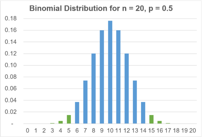
The critical values for the sign test come from a binomial distribution when the probability of a success is 50% since the median is the 50th percentile, and the sample size is 20.

If you were to calculate the discrete probability distribution for each possible value of $x$, you would get the following discrete probability distribution table (Figure 13-1) and corresponding graph (Figure 13-2).

Table of discrete probability distribution for each value of x between 0 and 20. The sum of the probabilities for x=0 through x=5 is 0.0206949, and the sum of the probabilities for x=15 through x=20 is 0.0206949. — Figure 13-1: Discrete probability distribution table for each value of $x$.

Binomial distribution bar graph for n=20, p=0.5. The bars for x=0 through x=5 and the bars for x=15 through x=20 are highlighted. — Figure 13-2: Graph of binomial distribution data from Figure 13-1, with the two tails highlighted.

When we add up the highlighted probabilities we would get a probability of approximately $0.0206949 + 0.0206949 = 0.0414$, which is below our alpha 0.05 for a two-tailed test. If we were to add in the values of $x = 6$ and $x = 14$ we would get 0.1153, which is above our value for alpha.

Figure 13-2 is a bar graph of showing the binomial distribution and shaded critical values. This means that $x = 5$ and $x = 15$ are the critical values for a two-tailed sign test with $n = 20$. If the test statistic is less than or equal to 5 or greater than or equal to 15, we would reject $H_{0}$.

The test statistic is the smaller of plus or minus signs, which is 2. Since $2 \leq 5$, we would reject $H_{0}$, which agrees with the p-value method.

If you were doing a one-tailed test you would use the probabilities for one of the tails.

A professor believes that a new online learning curriculum is increasing the median final exam score from the previous year, which was 75. A random sample of final exam scores were collected for students that went through the new curriculum. Test to see if the new curriculum is effective using $\alpha = 0.05$.

78 100 75 64 87 80 72 91 89 70 82 76

Solution

The hypotheses are:

$H_{0}:$ Median $= 75$
$H_{1}:$ Median $> 75$

Find the test statistic. Compare each value to the median. If the value is below the median then give it a negative sign, if the value is above the mean then give it a positive sign. If the value is tied with the median then give it a zero.

78
+

100
+

75
0

64
-

87
+

80
+

72
-

91
+

89
+

70
-

82
+

76
+

Count the number of positive and negative signs. Positive signs = 8, Negative signs = 3. The sample size is then $8 + 3 = 11$.

The test statistic for a right tailed test is the number of plus signs. Therefore, in this case, the test statistic is 8.

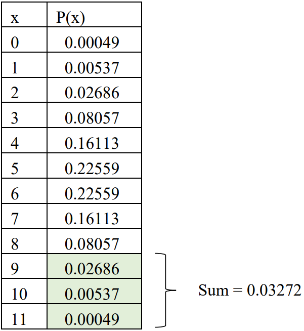
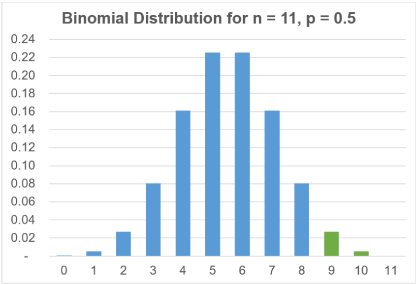
To find the critical value, use technology to find the probabilities for $x = 0$ to $x=11$ for a binomial distribution with $n = 11$ and $p = 0.5$. See Figure 13-3 for the results. Since $\alpha = 0.05$, add up the areas starting at the bottom at $x = 11$ until you get a sum of no more than 0.05.

$\text{P} (9 \leq X \leq 11) = \text{P}(X=9) + \text{P}(X=10) + \text{P}(X=11) = {}_{11} C_{10} \cdot 0.5^{9} \cdot 0.5^{2} + {}_{11} C_{10} \cdot 0.5^{10} \cdot 0.5^{1} + {}_{11} C_{11} \cdot 0.5^{0} \cdot 0.5^{11} = 0.03272.$

If we add in the next value of $\text{P}(X = 8) = 0.08057$, the sum would exceed 0.05, so we would stop at a critical value of $X = 9$. See Figure 13-4.

Discrete probability distribution table for values of x from 0 through 11. The sum of the probabilities for x=9, 10, and 11 is 0.03272. — Figure 13-3: Discrete probability distribution table for each value of $x$.

Bar graph of binomial distribution for n=11 and p=0.5. The bars for values of 9, 10, and 11 are highlighted. — Figure 13-4: Graph of binomial distribution data from Figure 13-3, with the right tail highlighted.

Since the test statistic $X = 8$ is not in the rejection area, we would fail to reject $H_{0}$.

At the 5% significance level, there is not enough evidence to support the claim that there is a statistically significant difference in final exam scores for the new online curriculum.

The median annual salary for high school teachers in the United States was $60,320. A teacher believes that the median high school salary in Oregon is significantly less than the national median. A sample of 100 high school teacher’s salaries found that 58 were below $60,320, 40 were above $60,320 and 2 were $60,320. Use $\alpha = 0.05$ to test their claim.

Solution

The hypotheses are:

$H_{0}:$ Median = $60,320
$H_{1}:$ Median < $60,320 (claim)

The sample size $n = 58 + 40 = 98$.

We will use $x = 58$. The p-value is found by taking $\text{P}(X \geq 58)$. This is a lot of work by hand, so use technology. For a TI-84 calculator use $1 - \text{binomcdf}(98, 0.5, 58) = 0.0272.$

On a TI-84 calculator, 1 minus the binomial cdf with inputs 98, 5, and 58 is 0.0271952788.

The p-value = 0.0427, which is less than $\alpha = 0.05$, so reject $H_{0}$.

There is enough evidence to support the claim that the median high school salary in Oregon is significantly less than the national median of $60,320.

The sign test can also be used for dependent samples when the assumptions for a paired t-test are not met.

A manufacturer believes that if routine maintenance (cleaning and oiling of machines) is increased to once a day rather than once a week, the number of defective parts produced by the machines will decrease. Nine machines are selected, and the number of defective parts produced over a 24-hour operating period is counted. Maintenance is then increased to once a day for a week, and the number of defective parts each machine produces is again counted over a 24-hour operating period. The data are shown here. At $\alpha = 0.05$, can the manufacturer conclude that the additional maintenance reduces the number of defective parts manufactured by the machines?

Machine 1 2 3 4 5 6 7 8 9 Before 6 18 5 4 16 13 20 9 3 After 5 16 7 4 18 12 14 7 1

Solution

$H_{0}:$ The additional maintenance does not reduce the number of defective parts manufactured by the machines.
$H_{1}:$ The additional maintenance reduces the number of defective parts manufactured by the machines.

Next, for each pair, take $\text{Before} - \text{After}$. If this difference is positive then put a $+$ sign next to it, if the difference is negative then put a $–$ sign next to it and if the difference is zero then put a 0 next to it.

Machine	1	2	3	4	5	6	7	8	9
Before	6	18	5	4	16	13	20	9	3
After	5	16	7	4	18	12	14	7	1
Sign of Difference	$+$	$+$	$-$	0	$-$	$+$	$+$	$+$	$+$

Count the number of positive and negative signs. Positive signs = 6, Negative signs = 2. The sample size is then $6 + 2 = 8$.

Note that this is a right-tailed test, since we are looking at “reducing” defective parts so that $\text{Before} > \text{After}$. The test statistic is the number of plus signs, $x = 6$.

$\text{P}(X \geq 6) = \text{P}(X=6) + \text{P}(X=7) + \text{P}(X=8) = {}_{8} C_{6} \cdot 0.5^{6} \cdot 0.5^{2} + {}_{8} C_{7} \cdot 0.5^{7} \cdot 0.5^{1} + {}_{8} C_{8} \cdot 0.5^{8} \cdot 0.5^{0} = 0.109375 + 0.031250 + 0.003906 = 0.144531$, which is the p-value.

For a TI calculator, use $1 - \text{binomcdf}(8, 0.5, 6) = 0.1445$. The p-value = 0.1445, which is greater than $\alpha = 0.05$; therefore do not reject $H_{0}$.

There is not enough evidence to support the claim that the additional maintenance reduces the number of defective parts manufactured by the machines.

Machine	1	2	3	4	5	6	7	8	9
Before	6	18	5	4	16	13	20	9	3
After	5	16	7	4	18	12	14	7	1
Sign of Difference	\(+\)	\(+\)	\(-\)	0	\(-\)	\(+\)	\(+\)	\(+\)	\(+\)