13.5: Mann-Whitney U Test

The Mann-Whitney U Test is the non-parametric alternative to the independent t-test. The test was expanded on Frank Wilcoxon’s Rank Sum test by Henry Mann and Donald Whitney.

Henry Mann

The independent t-test assumes the populations are normally distributed. When these conditions are not met, the Mann-Whitney Test is an alternative method.

If two groups come from the same distribution and were randomly assigned labels, then the two different groups should have values somewhat equally distributed between the two groups. The Mann-Whitney Test looks at all the possible rankings between the data points. For large sample sizes, a normal approximation of the distribution of ranks is used.

Small Sample Size Case \((n \leq 20)\)

Combine the data from both groups and sort from smallest to largest. Make sure to label the data values so you know which group they came from. Rank the data. Sum the ranks separately from each group. Let \(R_{1}\) = sum of ranks for group one and \(R_{2}\) = sum of ranks for group two.

Find the \(U\) statistic for both groups: \(U_{1} = R_{1} - \frac{n_{1} \left(n_{1}+1\right)}{2}, U_{2} = R_{2} - \frac{n_{2} \left(n_{2}+1\right)}{2}\).

The test statistic \(U = \text{Min} \left(U_{1}, U_{2}\right)\) is the smaller of \(U_{1}\) or \(U_{2}\). Critical values are found given in the tables in Figures 13-6 \((\alpha = 0.05)\) and 13-7 \((\alpha = 0.01)\).

Figure 13-8: Critical Values for 2-Tailed Mann-Whitney U Test for \(\alpha = 0.05\)

	\(n_{2}\)
\(n_{1}\)	2	3	4	5	6	7	8	9	10	11	12	13	14	15	16	17	18	19	20
2	-	-	-	-	-	-	0	0	0	0	1	1	1	1	1	2	2	2	2
3	-	-	-	0	1	1	2	2	3	3	4	4	5	5	6	6	7	7	8
4	-	-	0	1	2	3	4	4	5	6	7	8	9	10	11	11	12	13	13
5	-	0	1	2	3	5	6	7	8	9	11	12	13	14	15	17	18	19	20
6	-	1	2	3	5	6	8	10	11	13	14	16	17	19	21	22	24	25	27
7	-	1	3	5	6	8	10	12	14	16	18	20	22	24	26	28	30	32	34
8	0	2	4	6	8	10	13	15	17	19	22	24	26	29	31	34	36	38	41
9	0	2	4	7	10	12	15	17	21	23	26	28	31	34	37	39	42	45	48
10	0	3	5	8	11	14	17	20	23	26	29	33	36	39	42	45	48	52	55
11	0	3	6	9	13	16	19	23	26	30	33	37	40	44	47	51	55	58	62
12	1	4	7	11	14	18	22	26	29	33	37	41	45	49	53	57	61	65	69
13	1	4	8	12	16	20	24	28	33	37	41	45	50	54	59	63	67	72	76
14	1	5	9	13	17	22	26	31	36	40	45	50	55	59	64	67	74	78	83
15	1	5	10	14	19	24	29	34	39	44	49	54	59	64	70	75	80	85	90
16	1	6	11	15	21	26	31	37	42	47	53	59	64	70	75	81	86	92	98
17	2	6	11	17	22	28	34	39	45	51	57	63	67	75	81	87	93	99	105
18	2	7	12	18	24	30	36	42	48	55	61	67	74	80	86	93	99	106	112
19	2	7	13	19	25	32	38	45	52	58	65	72	78	85	92	99	106	113	119
20	2	8	14	20	27	34	41	48	55	62	69	76	83	90	98	105	112	119	127

Figure 13-9: Critical Values for 2-Tailed Mann-Whitney U Test for \(\alpha = 0.01\)

	\(n_{2}\)
\(n_{1}\)	2	3	4	5	6	7	8	9	10	11	12	13	14	15	16	17	18	19	20
2	-	-	-	-	-	-	-	-	-	-	-	-	-	-	-	-	-	0	0
3	-	-	-	-	-	-	-	0	0	0	1	1	1	2	2	2	2	3	3
4	-	-	-	-	0	0	1	1	2	2	3	3	4	5	5	6	6	7	8
5	-	-	-	0	1	1	2	3	4	5	6	7	7	8	9	10	11	12	13
6	-	-	0	1	2	3	4	5	6	7	9	10	11	12	13	15	16	17	18
7	-	-	0	1	3	4	6	7	9	10	12	13	15	16	18	19	21	22	24
8	-	-	1	2	4	6	7	9	11	13	15	17	18	20	22	24	26	28	30
9	-	0	1	3	5	7	9	11	13	16	18	20	22	24	27	29	31	33	36
10	-	0	2	4	6	9	11	13	16	18	21	24	26	29	31	34	37	39	42
11	-	0	2	5	7	10	13	16	18	21	24	27	30	33	36	39	42	45	46
12	-	1	3	6	9	12	15	18	21	24	27	31	34	37	41	44	47	51	54
13	-	1	3	7	10	13	17	20	24	27	31	34	38	42	45	49	53	56	60
14	-	1	4	7	11	15	18	22	26	30	34	38	42	46	50	54	58	63	67
15	-	2	5	8	12	16	20	24	29	33	37	42	46	51	55	60	64	69	73
16	-	2	5	9	13	18	22	27	31	36	41	45	50	55	60	65	70	74	79
17	-	2	6	10	15	19	24	29	34	39	44	49	54	60	65	70	75	81	86
18	-	2	6	11	16	21	26	31	37	42	47	53	58	64	70	75	81	87	92
19	0	3	7	12	17	22	28	33	39	45	51	56	63	69	74	81	87	93	99
20	0	3	8	13	18	24	30	36	42	46	54	60	67	73	79	86	92	99	105

If \(U\) is less than or equal to the critical value, then reject \(H_{0}\). Dashes indicate that the sample is too small to reject \(H_{0}\).

If you have only sample size above 20, use the following online calculator to find the critical value: https://www.socscistatistics.com/tests/mannwhitney/default.aspx.

Student employees are a major part of most college campus employment. Two major departments that participate in student hiring are listed below with the number of hours worked by students for a month. At the 0.05 level of significance, is there sufficient evidence to conclude a difference in hours between the two departments?

Athletics 20 24 17 12 18 22 25 30 15 19   Library 35 28 24 20 25 18 22 26 31 21 19

Solution

The hypotheses are:

\(H_{0}\): There is no difference in the number of hours student employees work for the athletics department and the library.
\(H_{1}\): There is a difference in the number of hours student employees work for the athletics department and the library.

Since the sample sizes are small and the distributions are not assumed to be normally distributed, the t-test for independent groups should not be used. Instead, we will use the nonparametric Mann-Whitney Test. To start, combine the groups, sort the data from smallest to largest, and note which group the data point is from.

Rank the data and look for the ties. Figure 13-10 shows the ranks for the combined data.

Figure 13-10: Ranks for combined and ordered data.

Student	Department	Hours	Rank
1	Athletics	12	1
2	Athletics	15	2
3	Athletics	17	3
4	Athletics	18	4.5
5	Library	18	4.5
6	Athletics	19	6.5
7	Library	19	6.5
8	Athletics	20	8.5
9	Library	20	8.5
10	Library	21	10
11	Athletics	22	11.5
12	Library	22	11.5
13	Athletics	24	13.5
14	Library	24	13.5
15	Athletics	25	15.5
16	Library	25	15.5
17	Library	26	17
18	Library	28	18
19	Athletics	30	19
20	Library	31	20
21	Library	35	21

Sum the ranks for each group:

\(R_{1} = 1 + 2 + 3 + 4.5 + 6.5 + 8.5 + 11.5 + 13.5 + 15.5 + 19 = 85\)

\(R_{2} = 4.5 + 6.5 +8.5 + 10 + 11.5 + 13.5 + 15.5 + 17 + 18 + 20 + 21 = 146\)

Compute the test statistic:

\(U_{1} = R_{1} - \frac{n_{1} \left(n_{1}+1\right)}{2} = 85 - \frac{10 \cdot 11}{2} = 30\)

\(U_{2} = R_{2} - \frac{n_{2} \left(n_{2}+1\right)}{2} = 146 - \frac{11 \cdot 12}{2} = 80\)

\(U = 30\)

Find the critical value using Figure 13-8, where \(n_{1} = 10\) and \(n_{2} = 11\). The critical value = 26.

Do not reject \(H_{0}\), since \(U = 30 > \text{CV} = 26\).

There is not enough evidence to support the claim that there is a difference in the number of hours student employees work for the athletics department and the library.

Large Sample Size Case (\(n_{1} > 20\) and \(n_{2} > 20\))

Find the \(U\) statistic for both groups: \(U_{1} = R_{1} - \frac{n_{1} \left(n_{1}+1\right)}{2}\), \(U_{2} = R_{2} - \frac{n_{2} \left(n_{2}+1\right)}{2}\).

Let \(U = \text{Min} \left(U_{1}, U_{2}\right)\), the smaller of \(U_{1}\) or \(U_{2}\). The formula for the test statistic is: \[z = \frac{\left(U - \left( \dfrac{n_{1} \cdot n_{2}}{2} \right)\right)}{\sqrt{\dfrac{n_{1} \cdot n_{2} \left(n_{1} + n_{2} + 1\right)}{12}}} \nonumber\]

A manager believes that the sales of coffee at their Portland store is more than the sales at their Cannon Beach store. They take a random sample of weekly sales from the two stores over the last year. Use the Mann-Whitney test to see if the manager’s claim could be true. Use the p-value method with \(\alpha = 0.05\).

Portland Cannon Beach 1510 1257   3585 1510 4125 4677   4399 5244 1510 3055   1764 1510 5244 1764   3853 4399 4125 6128   5244 1510 6128 3319   1510 5244 3319 6433   2533 4125 3319 5244   3585 2275 3055 6134   2533 2275 4025 3015   4399 3585       4125 5244\

Solution

Always choose group 1 as the group with the smallest sample size: in this case, Portland. (If the sample sizes are equal, then whatever group comes first in the problem is group one.) If there are no ties at the end, the last rank should match the total of both sample sizes.

Combine the data, keeping the group label, then rank the combined data.

Order	Store	Sales	Rank		Order	Store	Sales	Rank
1	Portland	1257	1		22	Cannon Beach	3585	21
2	Portland	1510	4.5		23	Cannon Beach	3853	23
3	Portland	1510	4.5		24	Portland	4025	24
4	Cannon Beach	1510	4.5		25	Portland	4125	26.5
5	Cannon Beach	1510	4.5		26	Portland	4125	26.5
6	Cannon Beach	1510	4.5		27	Cannon Beach	4125	26.5
7	Cannon Beach	1510	4.5		28	Cannon Beach	4125	26.5
8	Portland	1764	8.5		29	Cannon Beach	4399	30
9	Cannon Beach	1764	8.5		30	Cannon Beach	4399	30
10	Cannon Beach	2275	10.5		31	Cannon Beach	4399	30
11	Cannon Beach	2275	10.5		32	Portland	4677	32
12	Cannon Beach	2533	12.5		33	Portland	5244	35.5
13	Cannon Beach	2533	12.5		34	Portland	5244	35.5
14	Portland	3015	14		35	Cannon Beach	5244	35.5
15	Portland	3055	15.5		36	Cannon Beach	5244	35.5
16	Portland	3055	15.5		37	Cannon Beach	5244	35.5
17	Portland	3319	18		38	Cannon Beach	5244	35.5
18	Portland	3319	18		39	Portland	6128	39.5
19	Portland	3319	18		40	Portland	6128	39.5
20	Cannon Beach	3585	21		41	Portland	6134	41
21	Cannon Beach	3585	21		42	Portland	6433	42

The hypotheses are:

\(H_{0}\): There is no difference in the coffee sales between the Portland and Cannon Beach stores.
\(H_{1}\): There is a difference in the coffee sales between the Portland and Cannon Beach stores.

Sum the ranks for each group.

The sum for the Portland store’s ranks: \(R_{1} = 459.5\).
The sum for the Cannon Beach store’s ranks: \(R_{2} = 443.5\).

Compute the test statistic:

\(U_{1} = R_{1} - \frac{n_{1} \left(n_{1}+1\right)}{2} = 459.5 - \frac{20 \cdot 21}{2} = 249.5\)

\(U_{2} = R_{2} - \frac{n_{2} \left(n_{2}+1\right)}{2} = 443.5 - \frac{22 \cdot 23}{2} = 190.5\)

\(U = 190.5\)

\(z = \frac{190.5 - \left(\frac{20 \cdot 22}{2}\right)}{\sqrt{ \left(\frac{20 \cdot 22 (20 + 22 + 1)}{12}\right) }} = -0.7429\)

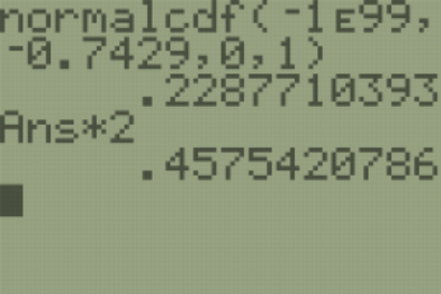
This test uses the standard normal distribution with the same technique for finding a p-value or critical value as the z-test performed in previous chapters. Compute the p-value for a standard normal distribution for \(z = -0.7429\) for a two-tailed test using \(2 * \text{normalcdf}(-1E99,-0.7429,0,1) = 0.4575\).

The p-value = \(0.4575 > \alpha = 0.05\); therefore, do not reject \(H_{0}\).

This is a two-tailed test with \(\alpha = 0.05\). Use the lower tail area of \(\alpha/2 = 0.05\) and you get critical values of \(z_{\alpha/2} = \pm 1.96\).

There is not enough evidence to support the claim that there is a difference in coffee sales between the Portland and Cannon beach stores.

There are no shortcut keys on the TI calculators or Excel for this Nonparametric Test. Note that if your data has tied ranks, there are several methods not addressed in this text, to correct the standard deviation. Hence, the z-score in some software packages may not match your results calculated by hand.