9.4: Two Variance or Standard Deviation F-Test

9.5.1 The F-Distribution

An F-distribution is another special type of distribution for a continuous random variable.

Properties of the F-distribution density curve:

• Right skewed.
• F-scores cannot be negative.
• The spread of an F-distribution is determined by the degrees of freedom of the numerator, and by the degrees of freedom of the denominator. The df are usually determined by the sample sizes of the two populations or number of groups.
• The total area under the curve is equal to 1 or 100%.

The shape of the distribution curve changes when the degrees of freedom change. Figure 9-9 shows examples of F-distributions with different degrees of freedom.

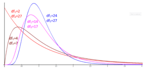
Figure 9-9

We will use the F-distribution in several types of hypothesis testing. For now, we are just learning how to find the critical value and probability using the F-distribution.

Use the TI-89 Distribution menu; or in Excel F.INV to find the critical values for the F-distribution for tail areas only, depending on the degrees of freedom. When finding a probability given an F-score, use the calculator Fcdf function under the DISTR menu or in Excel use F.DIST. Note that the TI-83 and TI-84 do not come with the INVF function, but you may be able to find the program online or from your instructor.

Alternatively, use the calculator at https://homepage.divms.uiowa.edu/~mbognar/applets/f.html which will also graph the distribution for you and shade in one tail at a time. You will see the shape of the F-distribution change in the following examples depending on the degrees of freedom used. For your own sketch just make sure you have a positively skewed distribution starting at zero.

The critical values F_\(\alpha\)/2 and F_{1–\(\alpha\)/2} are for a two-tailed test on the F-distribution curve with area 1 – \(\alpha\) between the critical values as shown in Figure 9-10. Note that the distribution starts at zero, is positively skewed, and never has negative F-scores.

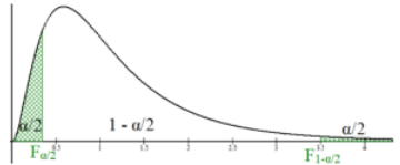
Figure 9-10

Compute the critical values F_\(\alpha\)/2 and F_{1–\(\alpha\)/2} with df₁ = 6 and df₂ = 14 for a two-tailed test, \(\alpha\) = 0.05.

Solution

Start by drawing the curve and finding the area in each tail. For this case, it would be an area of \(\alpha\)/2 in each tail. Then use technology to find the F-scores. Most technology only asks for the area to the left of the F-score you are trying to find. In Excel the function for F_\(\alpha\)/2 is F.INV(area in left-tail,df₁,df₂).

There is only one function, so use areas 0.025 and 0.975 in the left tail. For this example, we would have critical values F_0.025 = F.INV(0.025,6,14) = 0.1888 and F_0.975 = F.INV(0.975,6,14) = 3.5014. See Figure 9-11.

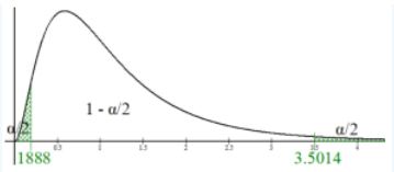
Figure 9-11

We have to calculate two distinct F-scores unlike symmetric distribution where we could just do ±z-score or ±t-score.

Note if you were doing a one-tailed test then do not divide alpha by two and use area = \(\alpha\) for a left-tailed test and area = 1 – \(\alpha\) for a right-tailed test.

Find the critical value for a right-tailed test with denominator degrees of freedom of 12 and numerator degrees of freedom of 2 with a 5% level of significance.

Solution

Draw the curve and shade in the top 5% of the upper tail since \(\alpha\) = 0.05, see Figure 9-12. When using technology, you will need the area to the left of the critical value that you are trying to find. This would be 1 – \(\alpha\) = 0.95. Then identify the degrees of freedom. The first degrees of freedom are the numerator df, therefore df₁ = 2. The second degrees of freedom are the denominator df, therefore df₂ = 12. Using Excel, we would have =F.INV(0.95,2,12) = 3.8853.

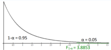
Figure 9-12

Compute P(F > 3.894), with df₁ = 3 and df₂ = 18

Solution

In Excel, use the function F.DIST(x,deg_freedom1,deg_freedom2,cumulative). Always use TRUE for the cumulative. The F.DIST function will find the probability (area) below F. Since we want the area above F we would need to also use the complement rule. The formula would be =1-F.DIST(3.894,3,18,TRUE) = 0.0263.

TI-84: The TI-84 calculator has a built in F-distribution. Press [2^nd] [DISTR] (this is F5: DISTR in the STAT app in the TI-89), then arrow down until you get to the Fcdf and press [Enter]. Depending on your calculator, you may not get a prompt for the boundaries and df. If you just see Fcdf( then you will need to enter each the lower boundary, upper boundary, df₁, and df₂ with a comma between each argument. The lower boundary is the 3.394 and the upper boundary is infinity (TI-83 and 84 use a really large number instead of ∞), then enter the two degrees of freedom. Press [Paste] and then [Enter], this will put the Fcdf(3.894,1E99,3,18) on your screen and then press [Enter] again to calculate the value.

Figure 9-13.

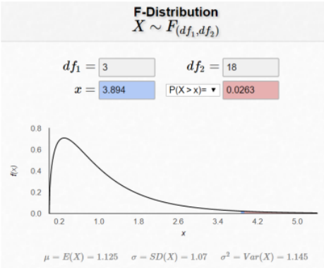
Figure 9-13

9.5.2 Hypothesis Test for Two Variances

Sometimes we will need to compare the variation or standard deviation between two groups. For example, let’s say that the average delivery time for two locations of the same company is the same but we hear complaint of inconsistent delivery times for one location. We can use an F-test to see if the standard deviations for the two locations was different.

There are three types of hypothesis tests for comparing the ratio of two population variances , see Figure 9-14.

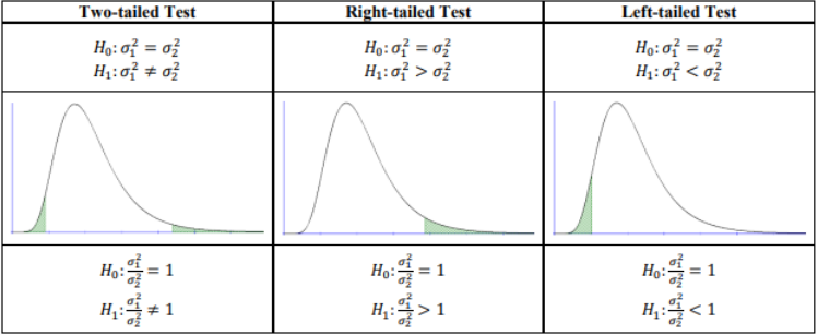
Figure 9-14

If we take the square root of the variance, we get a standard deviation. Therefore, taking the square root of both sides of the hypotheses, we can also use the same test for standard deviations. We use the following notation for the hypotheses.

There are 3 types of hypothesis tests for comparing the population standard deviations σ_1/σ₂, see Figure 9-15.

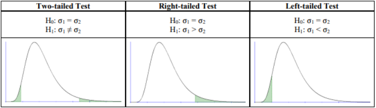
Figure 9-15

The F-test is a statistical test for comparing the variances or standard deviations from two populations.

The formula for the test statistic is \(F=\frac{s_{1}^{2}}{s_{2}^{2}}\).

With numerator degrees of freedom = Ndf = n₁ – 1, and denominator degrees of freedom = Ddf = n₂ – 1.

This test may only be used when both populations are independent and normally distributed.

Important: This F-test is not robust (a statistic is called “robust” if it still performs reasonably well even when the necessary conditions are not met). In particular, this F-test demands that both populations be normally distributed even for larger sample sizes. This F-test yields unreliable results when this condition is not met.

The traditional method (or critical value method), and the p-value method are performed with steps that are identical to those when performing hypothesis tests from previous sections.

A researcher claims that IQ scores of university students vary less than (have a smaller variance than) IQ scores of community college students. Based on a sample of 28 university students, the sample standard deviation 10, and for a sample of 25 community college students, the sample standard deviation 12. Test the claim using the traditional method of hypothesis testing with a level of significance \(\alpha\) = 0.05. Assume that IQ scores are normally distributed.

Solution

1. The claim is “IQ scores of university students (Group 1) have a smaller variance than IQ scores of community college students (Group 2).”

This is a left-tailed test; therefore, the hypotheses are: \(\begin{aligned}
&H_{0}: \sigma_{1}^{2}=\sigma_{2}^{2} \\
&H_{1}: \sigma_{1}^{2}<\sigma_{2}^{2}
\end{aligned}\).

2. We are using the F-test because we are performing a test about two population variances. We can use the F-test only if we assume that both populations are normally distributed. We will assume that the selection of each of the student groups was independent.

The problem gives us s₁ = 10, n₁ = 28, s₂ = 12, and n₂ = 25.

The formula for the test statistic is \(F=\frac{s_{1}^{2}}{s_{2}^{2}}=\frac{10^{2}}{12^{2}}=0.6944\).

3. The critical value for a left-tailed test with a level of significance \(\alpha\) = 0.05 is found using the invF program or Excel. See Figure 9-16.

Using Excel: The critical value is F_\(\alpha\) =F.INV(0.05,27,24) = 0.5182.

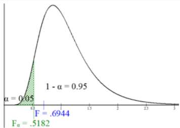
Figure 9-16

4. Decision: Compare the test statistic F = 0.6944 with the critical value F_\(\alpha\) = 0.5182, see Figure 9-16. Since the test statistic is not in the rejection region, we do not reject H₀.

5. Summary: There is not enough evidence to support the claim that the IQ scores of university students have a smaller variance than IQ scores of community college students.

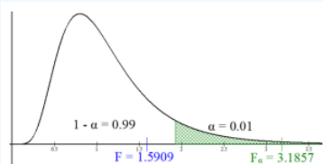
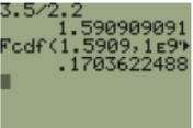
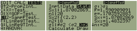
A random sample of 20 graduate college students and 18 undergraduate college students indicated these results concerning the amount of time spent in volunteer service per week. At \(\alpha\) = 0.01 level of significance, is there sufficient evidence to conclude that graduate students have a higher standard deviation of the number of volunteer hours per week compared to undergraduate students? Assume that number of volunteer hours per week is normally distributed.

  Graduate Undergraduate Sample Mean 3.8 2.5 Sample Variance 3.5 2.2 Sample Size 20 18

Solution

Assumptions: The two populations we are comparing are graduate and undergraduate college students. We are given that the number of volunteer hours per week is normally distributed. We are told that the samples were randomly selected and should therefore be independent.

Using the Traditional Method

1. We are trying to determine whether the standard deviation of the number of volunteer hours per week for graduate students (Group 1) is larger than undergraduate students (Group 2) or σ₁ > σ₂.

Therefore, the hypotheses are: \(\begin{aligned}
&\mathrm{H}_{0}: \sigma_{1}=\sigma_{2} \\
&\mathrm{H}_{1}: \sigma_{1}>\sigma_{2}
\end{aligned}\)

2. We are given that \(s_{1}^{2}\) =3.5, \(s_{2}^{2}\) = 2.3, n₁ =20 and n₂ =18. Note variances were given, so do not square the numbers again. The test statistic is, \(F=\frac{s_{1}^{2}}{s_{2}^{2}}=\frac{3.5}{2.2}=1.5909\).

3. Draw and label the distribution with the critical value for a right-tailed F-test with numerator degrees of freedom = n₁ – 1 = 19, and with denominator degrees of freedom = n₂ – 1 = 17. See Figure 9-17. Use right-tail area \(\alpha\) = 0.01 in Excel F_{1–\(\alpha\)} =F.INV.RT(0.01,19,17) to find the critical value 3.1857.

Figure 9-17

4. Decision: Since the test statistic is not in the rejection region, we do not reject H₀.

5. Summary: There is not enough evidence to support the claim that the population standard deviation of the number of volunteer hours per week for graduate college students is higher than undergraduate college students.

Using the p-value method

1. Step 1 remains the same.

Therefore, the hypotheses are: \(\begin{aligned}
&\mathrm{H}_{0}: \sigma_{1}=\sigma_{2} \\
&\mathrm{H}_{1}: \sigma_{1}>\sigma_{2}
\end{aligned}\)

2. Step 2 remains the same.

The test statistic is, \(F=\frac{s_{1}^{2}}{s_{2}^{2}}=\frac{3.5}{2.2}=1.5909\).

3. Compute the p-value using either the Fcdf on the calculator or Excel. If your test statistic is less than 1, then find the area to the left of the test statistic, if F is above 1 then find the area to the right of the test statistic. If you have a two-tailed test then double your tail area.

TI: Fcdf(lower,upper,df₁,df₂) = Fcdf(1.5909,1E99,19,17).

Excel: =F.DIST.RT(1.5909,19,17) = 0.1704.

4. Decision: Since the p-value = 0.1704 is greater than \(\alpha\) = 0.01, we “Do Not Reject H₀.”

5. Step 5, the summary remains the same. There is not enough evidence to support the claim that the population standard deviation of the number of volunteer hours per week for graduate college students is higher than undergraduate college students.

Alternatively use the following 2-Sample F-test shortcut on the TI calculator.

TI-84: Press the [STAT] key, arrow over to the [TESTS] menu, arrow down to the option [E:2-SampFTest] and press the [ENTER] key. Arrow over to the [Stats] menu and press the [Enter] key. Then type in the s₁, n₁, s₂, n₂, arrow over to the \(\neq\), <, > sign that is the same in the problem’s alternative hypothesis statement, then press the [ENTER] key, arrow down to [Calculate] and press the [ENTER] key. The calculator returns the test statistic F and the p-value.

Note: You have to put the standard deviation in the calculator, not the variance.

TI-89: Go to the [Apps] Stat/List Editor, then push 2^nd then F6 [Tests], then select 9: 2-SampFTest. Then type in the s₁, n₁, s₂, n₂ (or list names list1 & list2), select the sign \(\neq\), <, > that is the same in the problem’s alternative hypothesis statement, press the [ENTER] key to calculate. The calculator returns the F-test statistic and the p-value.

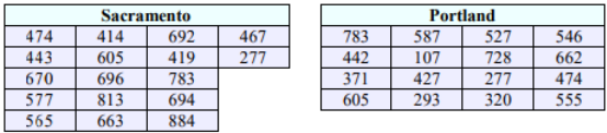
A researcher is studying the variability in electricity (in kilowatt hours) people from two different cities use in their homes. Random samples of 17 days in Sacramento and 16 days in Portland are given below. Test to see if there is a difference in the variance of electricity use between the two cities at α = 0.10. Assume that electricity use is normally distributed, use the p-value method.

Solution

The populations are independent and normally distributed.

The hypotheses are \(\begin{aligned}
&\mathrm{H}_{0}: \sigma_{1}^{2}=\sigma_{2}^{2} \\
&\mathrm{H}_{1}: \sigma_{1}^{2} \neq \sigma_{2}^{2}
\end{aligned}\)

Use technology to compute the standard deviations and sample sizes. Enter the Sacramento data into list 1, then do 1-Var Stats L1 and you should get s₁ = 163.2362 and n₁ = 17. Enter the Portland data into list 2, then do 1-Var Stats L2 and you should get s₂ = 179.3957 and n₂ = 16. Alternatively, use Excel’s descriptive statistics.

The test statistic is

The p-value would be double the area to the left of F = 0.82796 (Use double the area to the right if the test statistic is > 1).

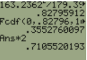
Using the TI calculator Fcdf(0,0.82796,16,15).

In Excel we get the p-value =2*F.DIST(E8,E7,F7,TRUE) = 0.7106.

Since the p-value is greater than alpha, we would fail to reject H₀.

There is no statistically significant difference between variance of electricity use between Sacramento and Portland.

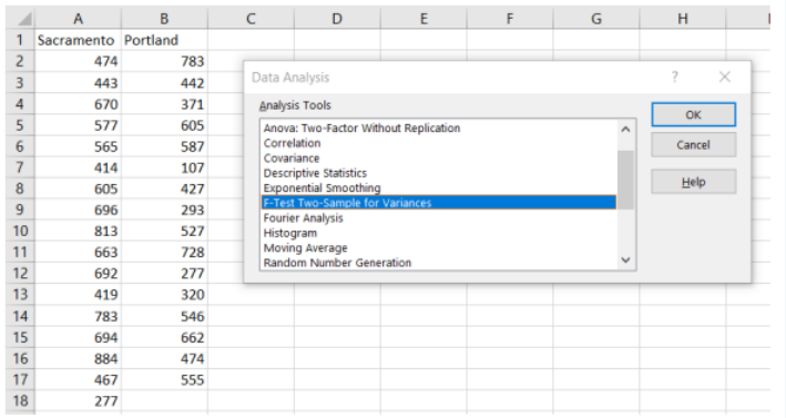
Excel: When you have raw data, you can use Excel to find all this information using the Data Analysis tool. Enter the data into Excel, then choose Data > Data Analysis > F-Test: Two Sample for Variances.

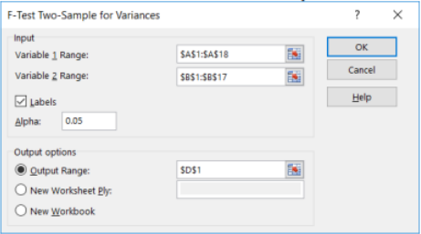
Enter the necessary information as we did in previous sections (see below) and select OK. Note that Excel only does a one-tail F-test so use \(\alpha\)/2 = 0.10/2 = 0.05 in the Alpha box.

We get the following output. Note you can only use the critical value in Excel for a left-tail test.

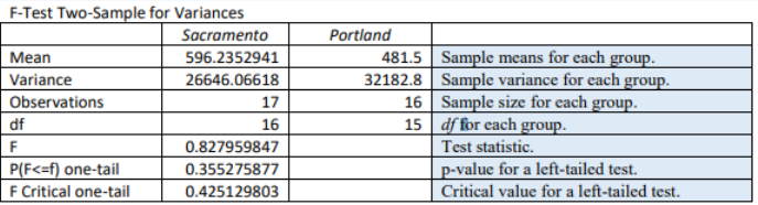
Excel for some reason only does the smaller tail area for the F-test, so you will need to double the p-value for a two-tailed test, p-value = 0.355275877*2 = 0.7106.