
6.5: The Central Limit Theorem
- Page ID
- 24047

The sample mean, denoted \(\overline{ x }\), is the average of a sample of a variable X. The sample mean is an estimate of the population mean µ. Every sample has a sample mean and these sample means differ (depending on the sample). Thus, before a sample is selected \(\overline{ x }\) is a variable, in fact, if the sample is a random sample then \(\overline{ x }\) is a random variable. For this reason, we can think of the “distribution of \(\overline{ x }\),” called the “Sampling Distribution of \(\overline{ x }\),” as the theoretical histogram constructed from the sample averages of all possible samples of size n.Definition: Word
Mean and Standard Deviation of a Sample Mean
Let \(\overline{ x }\) be the mean of a random sample of size n from a population having mean μ and standard deviation σ, then
The mean of the sample means = \(\mu_{\bar{x}}\) = µ.
The standard deviation (standard error) of the sample means = \(\sigma_{\bar{x}}=\frac{\sigma}{\sqrt{n}}\).
This says that the mean of the sample means is the same as the population mean. The standard deviation of the sample means is the population standard deviation divided by the square root of the sample size. This is called the sampling distribution of the mean.
Let X be the height of men in the United States. Studies show that the heights of 15-year old boys in the United States are normally distributed with average height 67 inches and a standard deviation of 2.5 inches. A random experiment consists of choosing 16 15-year old boys at random. Compute the mean and standard deviation of \(\overline{ x }\), that is, the mean and standard deviation for the average height of a random sample of 16 boys.
Solution
The mean of the sample means is the same as the population mean \(\mu_{\bar{x}}\) = 67.
The standard deviation in the sample means is the population standard deviation divided by the square root of the sample size, \(\sigma_{\bar{x}}=\frac{\sigma}{\sqrt{n}}=\frac{2.5}{\sqrt{16}}=0.625\).
Notice that the mean of a sample means is always the same as the mean of the population, but the standard deviation is smaller. See Figure 6-30.

Sampling Distribution of a Sample Mean
If a population is normally distributed N(µ, σ), then the sample mean \(\overline{ x }\) of n independent observations is normally distributed as \(N\left(\mu, \frac{\sigma}{\sqrt{n}}\right)\) /
Figure 6-31 shows three population distributions and the corresponding sampling distributions for sample sizes of 2, 5, 12 and 30. Notice as the sample size gets larger, the sampling distribution gets closer to the dashed red line of the normal distribution. Video explanation of this process: https://youtu.be/lsCc_pS3O28.
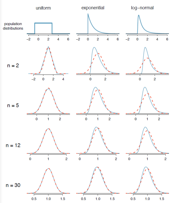
Retrieved from OpenIntroStatistics.
Figure 6-31
The Central Limit Theorem establishes that in some situations the distribution of the sample statistic will take on a normal distribution, even when the population is not normally distributed. This allows us to use the normal distribution to make inferences from samples to populations.
The Central Limit Theorem guarantees that the distribution of the sample mean will be normally distributed when the sample size is large (usually 30 or higher) no matter what shape the population distribution is.
Finding Probabilities Using the Central Limit Theorem (CLT)
If we are finding the probability of a sample mean and have a sample size of 30 or more, or the population was normally distributed, then we can use the normal distribution to find the probability that the sample mean is below, above or between two values using the CLT.
Watch this video on using this applet for the Central Limit Theorem, and then take some time to play with the applet to get a sense of the difference between the distribution of the population, the distribution of a sample and the sampling distribution.
Watch the video on how to use the applet: https://youtu.be/aIPvgiXyBMI.
Try the applet on your own. Applet: http://onlinestatbook.com/stat_sim/sampling_dist/index.html.
The population of midterm scores for all students taking a PSU Business Statistics course has a known standard deviation of 5.27. The mean of the population is 18.07 and the median of the population is 19. A sample of 25 was taken and the sample mean was 18.07 and we want to know what the sampling distribution for the mean looks like. Figure 6-32 shows 3 graphs using the Sampling Distribution Applet.
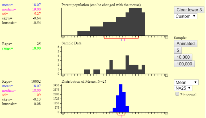
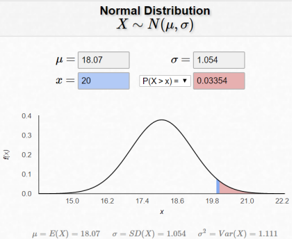
a) What is the mean and standard deviation of the sampling distribution? b) Would you expect midterm exam scores to be skewed or bell-shaped? c) Which of these graphs in Figure 6-32 correspond to the distribution of the population, distribution of a single sample and the sampling distribution of the mean? d) Compute the probability that for next term’s class they have a sample mean of more than 20. a) By the Central Limit Theorem (CLT) the mean of the sampling distribution \(\mu_{\bar{x}}\) equals the mean of the population which was given as µ=18.07. The standard deviation of the sampling distribution by the CLT would be the population standard deviation divided by the square root of the sample size \(\sigma_{\bar{x}}=\frac{\sigma}{\sqrt{n}}=\frac{5.27}{\sqrt{25}}=1.054\) b) The population mean = 18.07 is smaller than the median = 19 therefore the distribution is negatively skewed, the mean is pulled in the direction of the outliers. c) Using the Sampling Distribution Applet and the CLT, the sampling distribution will be bell-shaped therefore, graph 3 has to be the sampling distribution. Graphs 1 & 2 in Figure 6-32 are both negatively skewed. A single sample of 25 should look similar to the entire population, but we would expect only 25 items and not every score possible would be received from the 25 students. Graph 1 in Figure 6-32 fits this description and therefore the graph of the distribution of a single sample (which is not the same thing as the sampling distribution) is graph 1. This leaves graph 2 as the distribution of the population. Figure 6-33 is a picture of the applet modeling the exam scores. Note the top picture is the population distribution, the second graph is simulating a single sample drawn and the bottom picture is a graph of all the sample means for each sample. This last graph is the sampling distribution of the means. d) The P(\(\bar{X}\) > 20) would be normally distributed with a mean \(\mu_{\bar{x}}\) = 18.07 with a standard deviation of \(\sigma_{\bar{x}}=\frac{\sigma}{\sqrt{n}}=\frac{5.27}{\sqrt{25}}=1.054\) Draw and shade the sampling distribution curve. This calculator can be used to draw and shade the sampling distribution: http://homepage.divms.uiowa.edu/~mbognar/applets/normal.html, filling in the mean μ, standard deviation \(\frac{\sigma}{\sqrt{n}}\) and x-value (in this case the sample mean) will find the probability. See Figure 6-34. TI Calculator: normalcdf(20,1E99,18.07,5.27/√25) = 0.0335. Excel: P(\(\bar{X}\) > 20) =1-NORM.DIST(20,18.07,5.27/SQRT(25),TRUE) = 0.0335.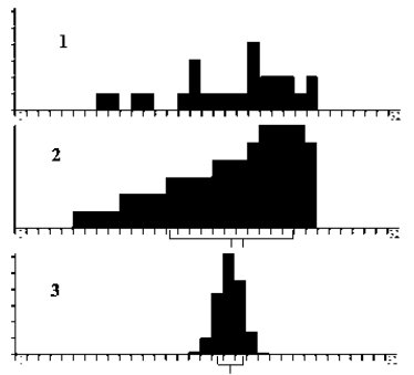
Solution
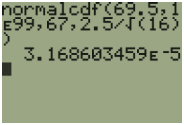
Let X be the height of 15-year old boys in the United States. Studies show that the heights of 15-year old boys in the United States are normally distributed with average height of 67 inches and a standard deviation of 2.5 inches. A random experiment consists of randomly choosing sixteen 15-year old boys. Compute the probability that the mean height of those sampled is 69.5 inches or taller.
Solution
The sample mean \(\mu_{\bar{x}}\) is approximately \(N(67,0.625) . \mathrm{P}(\bar{X} \geq 69.5)=P\left(\frac{8-67}{0.625} \geq \frac{69.5-67}{0.625}\right)=\mathrm{P}(Z \geq 4) \approx 0.00003\), using the calculator, be careful with the scientific notation. This is a very small probability.
This should make sense because one would think that the likelihood of randomly selecting 16 boys that have an average height of 5’9.5” would be slim.
Figure 6-35 shows the density curves showing the shaded areas of P(X ≥ 69.5) and P(\(\mu_{\bar{x}}\) ≥ 69.5).

The sampling distribution has a much smaller spread (standard deviation) and hence less area to the right of 69.5.
In general, the Central Limit Theorem questions will use the same method as previous sections, however you will use a standard deviation of \(\frac{\sigma}{\sqrt{n}}\) and a z-score of \(z=\frac{\bar{x}-\mu}{\left(\frac{\sigma}{\sqrt{n}}\right)}\).
The average teacher’s salary in Connecticut (ranked first among states) is $57,337. Suppose that the distribution of salaries is normally distributed with a standard deviation of $7,500.
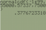
a) What is the probability that a randomly selected teacher makes less than $55,000 per year?
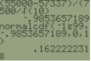
b) If we sample 10 teachers’ salaries, what is the probability that the sample mean is less than $55,000?
c) If we sample 100 teachers’ salaries, what is the probability that the sample mean is less than $55,000?
Solution
a) Find P(X < 55000), since we are only looking at one person use \(z=\frac{x-\mu}{\sigma}\). If we were asked to standardize the salary, \(z=\frac{55000-57337}{7500}=-0.3116\), however we can use technology and skip this step.
Use the normalcdf(-1E99,55000,57337,7500) (the TI-89 use -∞ for the lower boundary instead of -1E99) and you get the probability of 0.3777. The P(X < 55000) = P(Z < –0.3116) = 0.3777.
Note that we are not using the CLT since we are not finding the probability of an average for a group of people, just the probability for one person.
b) Find P(\(\mu_{\bar{x}}\) < 55000), but we are looking at the probability of a mean for 10 teachers, so use \(z=\frac{\bar{x}-\mu}{\left(\frac{\sigma}{\sqrt{n}}\right)}\). Standardize the salary, \(z=\frac{55000-57337}{\left(\frac{7500}{\sqrt{10}}\right)}=–0.9853657189\), use your calculator to get P(\(\mu_{\bar{x}}\) < 55000) = P(Z < –0.9853657189) = 0.1622.
You do not need the extra step of finding the z-score first. Instead you can use normalcdf(-1E99,55000,57337,7500/√10) = 0.1622.
c) Find P(\(\mu_{\bar{x}}\) < 55000), but we are looking at the probability of a mean for 100 teachers, so use \(z=\frac{\bar{x}-\mu}{\left(\frac{\sigma}{\sqrt{n}}\right)}\). Standardize the salary, \(z=\frac{55000-57337}{\left(\frac{7500}{\sqrt{100}}\right)}=–3.116\) use your calculator normalcdf(-1E99,55000,57337,7500/√100) to get P(\(\mu_{\bar{x}}\) < 55000) = P(Z < –3.116) = 0.0009167.
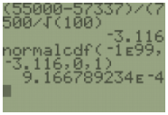
As the sample size increase, the probability of seeing a sample mean of less than $55,000 is getting smaller.
When you have a z-score that is less than –3 or greater than 3 we would call this a rare event or outlier. We will use this same process in inferential statistics in chapter 8.