6.1: Introductions

Last updated
Save as PDF

Page ID: 24043

\( \newcommand{\vecs}[1]{\overset { \scriptstyle \rightharpoonup} {\mathbf{#1}} } \) \( \newcommand{\vecd}[1]{\overset{-\!-\!\rightharpoonup}{\vphantom{a}\smash {#1}}} \)\(\newcommand{\id}{\mathrm{id}}\) \( \newcommand{\Span}{\mathrm{span}}\) \( \newcommand{\kernel}{\mathrm{null}\,}\) \( \newcommand{\range}{\mathrm{range}\,}\) \( \newcommand{\RealPart}{\mathrm{Re}}\) \( \newcommand{\ImaginaryPart}{\mathrm{Im}}\) \( \newcommand{\Argument}{\mathrm{Arg}}\) \( \newcommand{\norm}[1]{\| #1 \|}\) \( \newcommand{\inner}[2]{\langle #1, #2 \rangle}\) \( \newcommand{\Span}{\mathrm{span}}\) \(\newcommand{\id}{\mathrm{id}}\) \( \newcommand{\Span}{\mathrm{span}}\) \( \newcommand{\kernel}{\mathrm{null}\,}\) \( \newcommand{\range}{\mathrm{range}\,}\) \( \newcommand{\RealPart}{\mathrm{Re}}\) \( \newcommand{\ImaginaryPart}{\mathrm{Im}}\) \( \newcommand{\Argument}{\mathrm{Arg}}\) \( \newcommand{\norm}[1]{\| #1 \|}\) \( \newcommand{\inner}[2]{\langle #1, #2 \rangle}\) \( \newcommand{\Span}{\mathrm{span}}\)\(\newcommand{\AA}{\unicode[.8,0]{x212B}}\)

A continuous random variable (usually denoted as X) is a variable that has an infinite number of random values in an interval of numbers. There are many different types of continuous distributions. To be a valid continuous distribution the total area under the curve has to be equal to one and the function’s y-values need to be positive.

For example, we may have a random variable that is uniformly distributed so we could use the Uniform distribution that looks like a rectangle. See Figure 6-1.

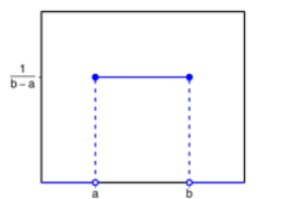
Figure 6-1

We may want to model the time it takes customer service to complete a call with the exponential distribution. See Figure 6-2.

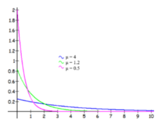
Figure 6-2

We may have standardized test scores that follow a bell-shaped curve like the Gaussian (Normal) Distribution. See Figure 6-3.

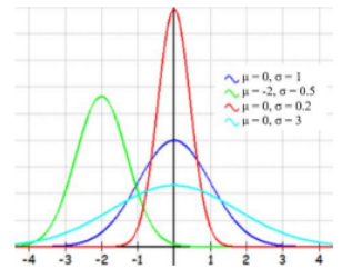
Figure 6-3

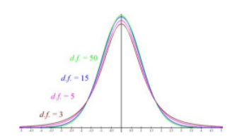
Figure 6-4

We may want to model the average time it takes for a component to be manufactured and use the bell-shaped Student t-distribution. See Figure 6-4.

This is just an introductory course so we are only going to cover a few distributions. If you want to explore more distributions, check out the chart by Larry Leemis at: http://www.math.wm.edu/~leemis/chart/UDR/UDR.html.

Very Important

The probability of an interval between two X values is equal to the area under the density curve between those two \(X\) values. For a discrete random variable, we can assign probabilities to each outcome. We cannot do this for a continuous random variable. The probability for a single \(X\) value for a continuous random variable is 0. Thus “” are equivalent to “≤” and “≥.” In other words,

\[P(a ≤ X ≤ b) = P(a < X < b) = P(a ≤ X < b) = P(a < X ≤ b) \nonumber\]

since there is no area of a line.

We now will look at some specific models that have been found useful in practice. Consider an experiment that consists of observing events in a certain time frame, such as buses arriving at a bus stop or telephone calls coming into a switchboard during a specified period. It may then be of interest to place a probability distribution on the actual time of occurrence. In this section, we will tell you which distribution to use in the question.