6.3: Exponential Distribution

Last updated
Save as PDF

Page ID: 24045

\( \newcommand{\vecs}[1]{\overset { \scriptstyle \rightharpoonup} {\mathbf{#1}} } \) \( \newcommand{\vecd}[1]{\overset{-\!-\!\rightharpoonup}{\vphantom{a}\smash {#1}}} \)\(\newcommand{\id}{\mathrm{id}}\) \( \newcommand{\Span}{\mathrm{span}}\) \( \newcommand{\kernel}{\mathrm{null}\,}\) \( \newcommand{\range}{\mathrm{range}\,}\) \( \newcommand{\RealPart}{\mathrm{Re}}\) \( \newcommand{\ImaginaryPart}{\mathrm{Im}}\) \( \newcommand{\Argument}{\mathrm{Arg}}\) \( \newcommand{\norm}[1]{\| #1 \|}\) \( \newcommand{\inner}[2]{\langle #1, #2 \rangle}\) \( \newcommand{\Span}{\mathrm{span}}\) \(\newcommand{\id}{\mathrm{id}}\) \( \newcommand{\Span}{\mathrm{span}}\) \( \newcommand{\kernel}{\mathrm{null}\,}\) \( \newcommand{\range}{\mathrm{range}\,}\) \( \newcommand{\RealPart}{\mathrm{Re}}\) \( \newcommand{\ImaginaryPart}{\mathrm{Im}}\) \( \newcommand{\Argument}{\mathrm{Arg}}\) \( \newcommand{\norm}[1]{\| #1 \|}\) \( \newcommand{\inner}[2]{\langle #1, #2 \rangle}\) \( \newcommand{\Span}{\mathrm{span}}\)\(\newcommand{\AA}{\unicode[.8,0]{x212B}}\)

An exponential distribution models a continuous random variable over time, area or space where the rate of occurrences decreases as X gets larger.

The probability density function (PDF) for an exponential curve is

\[f(x)= \{\begin{array}{l}\lambda e^{-x \lambda}, \text {for } x \geq 0 \\ 0, \text{elsewhere}\end{array}.\]

The value lambda λ is the fixed rate of occurrence and is equal to one divided by the mean, \(\frac{1}{\mu}\).

If the mean is given in the problem then you write the PDF as f(x)= \(\frac{1}{\mu} e^{\left(-\frac{x}{\mu}\right)}\), where e is a mathematical constant approximately equal to 2.71828, x ≥ 0 and x is the value you are trying to find the probability for, μ is the mean number of a successes over an interval of time, space, volume, etc. The distribution is denoted as X~Exp(λ).

Figure 6-8 gives example graphs for a mean of 5, 10 and 20. Note the curve hits the y-axis at 1/μ and keeps going forever to the right with an asymptote at y = 0.

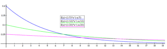
Figure 6-8

You would need integral calculus skills to find the area under this curve. To get around having the calculus requirement, we have three scenarios that we can use to find probability for an exponential distribution where we will not have to use the PDF.

To find the probability (area) under the exponential curve, use the following formulas.

\(\mathrm{P}(X \geq x)=\mathrm{P}(X>x)=\mathrm{e}^{-x / \mu}\)
\(\mathrm{P}(X \leq x)=\mathrm{P}(X<x)=1-\mathrm{e}^{-x / \mu}\)
\(\mathrm{P}\left(x_{1} \leq X \leq x_{2}\right)=\mathrm{P}\left(x_{1}<X<x_{2}\right)=e^{\left(-x_{1} / \mu\right)}-e^{\left(-x_{2} / \mu\right)}\)

The time it takes to help a customer at the customer service desk is exponentially distributed with an average help time of 45 seconds. Find the probability that a customer waits less than two minutes.

Solution

We need to have the same units as the mean in the question so instead of finding P(X < 2 minutes) we will use P(X < 120 seconds). Also note that < and ≤ find the same probabilities so use the equation \(\mathrm{P}(X

\[\mathrm{P}(X<120)=1-\mathrm{e}^{-120 / 45}=0.9305. \nonumber\]

In Excel use =EXPON.DIST(x,λ,TRUE) =EXPON.DIST(120,1/45,TRUE) = 0.9305.

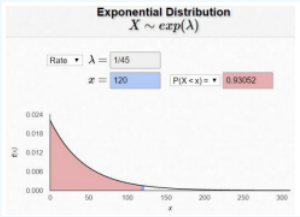
Figure 6-9

Alternatively, as shown in Figure 6-9, the following website will calculate the exponential probability: https://homepage.divms.uiowa.edu/~mbognar/applets/exp.html.