4.3: Complement Rule

Last updated
Save as PDF

Page ID: 24035

$ \newcommand{\vecs}[1]{\overset { \scriptstyle \rightharpoonup} {\mathbf{#1}} } $ $ \newcommand{\vecd}[1]{\overset{-\!-\!\rightharpoonup}{\vphantom{a}\smash {#1}}} $$\newcommand{\id}{\mathrm{id}}$ $ \newcommand{\Span}{\mathrm{span}}$ $ \newcommand{\kernel}{\mathrm{null}\,}$ $ \newcommand{\range}{\mathrm{range}\,}$ $ \newcommand{\RealPart}{\mathrm{Re}}$ $ \newcommand{\ImaginaryPart}{\mathrm{Im}}$ $ \newcommand{\Argument}{\mathrm{Arg}}$ $ \newcommand{\norm}[1]{\| #1 \|}$ $ \newcommand{\inner}[2]{\langle #1, #2 \rangle}$ $ \newcommand{\Span}{\mathrm{span}}$ $\newcommand{\id}{\mathrm{id}}$ $ \newcommand{\Span}{\mathrm{span}}$ $ \newcommand{\kernel}{\mathrm{null}\,}$ $ \newcommand{\range}{\mathrm{range}\,}$ $ \newcommand{\RealPart}{\mathrm{Re}}$ $ \newcommand{\ImaginaryPart}{\mathrm{Im}}$ $ \newcommand{\Argument}{\mathrm{Arg}}$ $ \newcommand{\norm}[1]{\| #1 \|}$ $ \newcommand{\inner}[2]{\langle #1, #2 \rangle}$ $ \newcommand{\Span}{\mathrm{span}}$$\newcommand{\AA}{\unicode[.8,0]{x212B}}$

AA random sample of 500 records from the 2010 United States Census were downloaded to Excel and the following contingency table was found for biological sex and marital status. Select one member at random and find the following probabilities.

Count of Marital StatusColumn Labels Row LabelsFemaleMaleGrand Total Divorced 21 17 38 Married/spouse absent 5 9 14 Married/spouse absent 92 100 192 Never married/single 93 129 222 Separated 1 2 3 Widowed 20 11 31 Grand Total232268500

a) Compute the probability that a person is divorced.

b) Compute the probability that a person is not divorced.

Solution

a) Take the row total of all divorced which is 38 and then divide by the grand total of 500 to get P(Divorced) = 38/500 = 0.076.

b) We can add up all the other category totals besides divorced 14 + 192 + 222 + 3 + 31 = 462, then divide by the grand total to get P(Not Divorced) = 462/500 = 0.924.

There is a faster way to computer these probabilities that will be important for more complicated probabilities called the complement rule. The table contains 100% (100% = 1 as a proportion) of our data so we can assume that the probability of the divorced is the opposite (complement) to the probability of not being divorced.

Notice that the P(Divorced) + P(Not Divorced) = 1. This is because these two events have no outcomes in common, and together they make up the entire sample space. Events that have this property are called complementary events. Notice P(Not Divorced) = 1 – P(Divorced) = 1 – 0.076 = 0.924.

If two events are complementary events, then to find the probability of one event just subtract the probability from 1. Notation used for complement of A also called “not A” is A^C.

P(A) + P(A^C) = 1 or P(A) = 1 – P(A^C) or P(A^C) = 1 – P(A)

Some texts will use the notation for a complement as A' or $\overline{ A }$, instead of A^C.

Suppose you know that the probability of it raining today is 80%. What is the probability of it not raining today?

Solution

Since not raining is the complement of raining, then P(not raining) = 1 – P(raining) = 1 – 0.8 = 0.2.

“On a small obscure world somewhere in the middle of nowhere in particular - nowhere, that is, that could ever be found, since it is protected by a vast field of unprobability to which only six men in this galaxy have a key - it was raining.” (Adams, 2002)

Venn Diagrams

Figure 4-5 is an example of a Venn diagram and is a visual way to represent sets and probability. The rectangle represents all the possible outcomes in the entire sample space (the population). The shapes inside the rectangle represent each event in the sample space. Usually these are ovals, but they can be any shape you want. If there are any shared elements between the events then the circles should overlap one another.

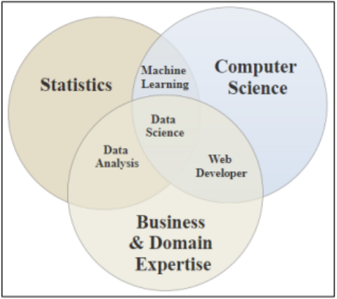
Figure 4-5

The field of statistics includes machine learning, data analysis, and data science. The field of computer science includes machine learning, data science and web development. The field of business and domain expertise includes data analysis, data science and web development. If you know machine learning, then you will need a background in both statistics and computer science. If you are a data scientist, then you will need a background in statistics, computer science, business and domain expertise.

Suppose you know the probability of not getting the flu is 0.24. Draw a Venn diagram and find the probability of getting the flu.

Solution

Since getting the flu is the complement of not getting the flu, the P(getting the flu) = 1 – P(not getting the flu) = 1 – 0.24 = 0.76.

Label each space as in Figure 4-6.

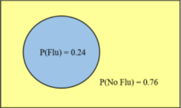
Figure 4-6

The complement is useful when you are trying to find the probability of an event that involves the words “at least” or an event that involves the words “at most.” As an example of an “at least” event is supposing you want to find the probability of making at least $50,000 when you graduate from college. That means you want the probability of your salary being greater than or equal to $50,000.

An example of an “at most” event is supposing you want to find the probability of rolling a die and getting at most a 4. That means that you want to get less than or equal to a 4 on the die, a 1, 2, 3, or 4.

The reason to use the complement is that sometimes it is easier to find the probability of the complement and then subtract from 1.