4.6: Conditional Probability
- Page ID
- 26011
\( \newcommand{\vecs}[1]{\overset { \scriptstyle \rightharpoonup} {\mathbf{#1}} } \)
\( \newcommand{\vecd}[1]{\overset{-\!-\!\rightharpoonup}{\vphantom{a}\smash {#1}}} \)
\( \newcommand{\dsum}{\displaystyle\sum\limits} \)
\( \newcommand{\dint}{\displaystyle\int\limits} \)
\( \newcommand{\dlim}{\displaystyle\lim\limits} \)
\( \newcommand{\id}{\mathrm{id}}\) \( \newcommand{\Span}{\mathrm{span}}\)
( \newcommand{\kernel}{\mathrm{null}\,}\) \( \newcommand{\range}{\mathrm{range}\,}\)
\( \newcommand{\RealPart}{\mathrm{Re}}\) \( \newcommand{\ImaginaryPart}{\mathrm{Im}}\)
\( \newcommand{\Argument}{\mathrm{Arg}}\) \( \newcommand{\norm}[1]{\| #1 \|}\)
\( \newcommand{\inner}[2]{\langle #1, #2 \rangle}\)
\( \newcommand{\Span}{\mathrm{span}}\)
\( \newcommand{\id}{\mathrm{id}}\)
\( \newcommand{\Span}{\mathrm{span}}\)
\( \newcommand{\kernel}{\mathrm{null}\,}\)
\( \newcommand{\range}{\mathrm{range}\,}\)
\( \newcommand{\RealPart}{\mathrm{Re}}\)
\( \newcommand{\ImaginaryPart}{\mathrm{Im}}\)
\( \newcommand{\Argument}{\mathrm{Arg}}\)
\( \newcommand{\norm}[1]{\| #1 \|}\)
\( \newcommand{\inner}[2]{\langle #1, #2 \rangle}\)
\( \newcommand{\Span}{\mathrm{span}}\) \( \newcommand{\AA}{\unicode[.8,0]{x212B}}\)
\( \newcommand{\vectorA}[1]{\vec{#1}} % arrow\)
\( \newcommand{\vectorAt}[1]{\vec{\text{#1}}} % arrow\)
\( \newcommand{\vectorB}[1]{\overset { \scriptstyle \rightharpoonup} {\mathbf{#1}} } \)
\( \newcommand{\vectorC}[1]{\textbf{#1}} \)
\( \newcommand{\vectorD}[1]{\overrightarrow{#1}} \)
\( \newcommand{\vectorDt}[1]{\overrightarrow{\text{#1}}} \)
\( \newcommand{\vectE}[1]{\overset{-\!-\!\rightharpoonup}{\vphantom{a}\smash{\mathbf {#1}}}} \)
\( \newcommand{\vecs}[1]{\overset { \scriptstyle \rightharpoonup} {\mathbf{#1}} } \)
\(\newcommand{\longvect}{\overrightarrow}\)
\( \newcommand{\vecd}[1]{\overset{-\!-\!\rightharpoonup}{\vphantom{a}\smash {#1}}} \)
\(\newcommand{\avec}{\mathbf a}\) \(\newcommand{\bvec}{\mathbf b}\) \(\newcommand{\cvec}{\mathbf c}\) \(\newcommand{\dvec}{\mathbf d}\) \(\newcommand{\dtil}{\widetilde{\mathbf d}}\) \(\newcommand{\evec}{\mathbf e}\) \(\newcommand{\fvec}{\mathbf f}\) \(\newcommand{\nvec}{\mathbf n}\) \(\newcommand{\pvec}{\mathbf p}\) \(\newcommand{\qvec}{\mathbf q}\) \(\newcommand{\svec}{\mathbf s}\) \(\newcommand{\tvec}{\mathbf t}\) \(\newcommand{\uvec}{\mathbf u}\) \(\newcommand{\vvec}{\mathbf v}\) \(\newcommand{\wvec}{\mathbf w}\) \(\newcommand{\xvec}{\mathbf x}\) \(\newcommand{\yvec}{\mathbf y}\) \(\newcommand{\zvec}{\mathbf z}\) \(\newcommand{\rvec}{\mathbf r}\) \(\newcommand{\mvec}{\mathbf m}\) \(\newcommand{\zerovec}{\mathbf 0}\) \(\newcommand{\onevec}{\mathbf 1}\) \(\newcommand{\real}{\mathbb R}\) \(\newcommand{\twovec}[2]{\left[\begin{array}{r}#1 \\ #2 \end{array}\right]}\) \(\newcommand{\ctwovec}[2]{\left[\begin{array}{c}#1 \\ #2 \end{array}\right]}\) \(\newcommand{\threevec}[3]{\left[\begin{array}{r}#1 \\ #2 \\ #3 \end{array}\right]}\) \(\newcommand{\cthreevec}[3]{\left[\begin{array}{c}#1 \\ #2 \\ #3 \end{array}\right]}\) \(\newcommand{\fourvec}[4]{\left[\begin{array}{r}#1 \\ #2 \\ #3 \\ #4 \end{array}\right]}\) \(\newcommand{\cfourvec}[4]{\left[\begin{array}{c}#1 \\ #2 \\ #3 \\ #4 \end{array}\right]}\) \(\newcommand{\fivevec}[5]{\left[\begin{array}{r}#1 \\ #2 \\ #3 \\ #4 \\ #5 \\ \end{array}\right]}\) \(\newcommand{\cfivevec}[5]{\left[\begin{array}{c}#1 \\ #2 \\ #3 \\ #4 \\ #5 \\ \end{array}\right]}\) \(\newcommand{\mattwo}[4]{\left[\begin{array}{rr}#1 \amp #2 \\ #3 \amp #4 \\ \end{array}\right]}\) \(\newcommand{\laspan}[1]{\text{Span}\{#1\}}\) \(\newcommand{\bcal}{\cal B}\) \(\newcommand{\ccal}{\cal C}\) \(\newcommand{\scal}{\cal S}\) \(\newcommand{\wcal}{\cal W}\) \(\newcommand{\ecal}{\cal E}\) \(\newcommand{\coords}[2]{\left\{#1\right\}_{#2}}\) \(\newcommand{\gray}[1]{\color{gray}{#1}}\) \(\newcommand{\lgray}[1]{\color{lightgray}{#1}}\) \(\newcommand{\rank}{\operatorname{rank}}\) \(\newcommand{\row}{\text{Row}}\) \(\newcommand{\col}{\text{Col}}\) \(\renewcommand{\row}{\text{Row}}\) \(\newcommand{\nul}{\text{Nul}}\) \(\newcommand{\var}{\text{Var}}\) \(\newcommand{\corr}{\text{corr}}\) \(\newcommand{\len}[1]{\left|#1\right|}\) \(\newcommand{\bbar}{\overline{\bvec}}\) \(\newcommand{\bhat}{\widehat{\bvec}}\) \(\newcommand{\bperp}{\bvec^\perp}\) \(\newcommand{\xhat}{\widehat{\xvec}}\) \(\newcommand{\vhat}{\widehat{\vvec}}\) \(\newcommand{\uhat}{\widehat{\uvec}}\) \(\newcommand{\what}{\widehat{\wvec}}\) \(\newcommand{\Sighat}{\widehat{\Sigma}}\) \(\newcommand{\lt}{<}\) \(\newcommand{\gt}{>}\) \(\newcommand{\amp}{&}\) \(\definecolor{fillinmathshade}{gray}{0.9}\)The probability of event B happening, given that event A already happened, is called the conditional probability. The conditional probability of B, given A is written as P(B | A), and is read as “the probability of B given A happened first.” We can use the General Multiplication Rule when two events are dependent.
\[\begin{align*} P(A ∩ B) &= P(A) \cdot P(B | A) P(A ∩ B) \\[4pt] &= P(A) \cdot P(B|A) \end{align*}\]
A bag contains 10 colored marbles: 7 red and 3 blue. A random experiment consists of drawing a marble from the bag, then drawing another marble without replacement (without putting the first marble back in the bag). Find the probability of drawing a red marble on the first draw (event R1), and drawing another red marble on the second draw (event R2).
Solution
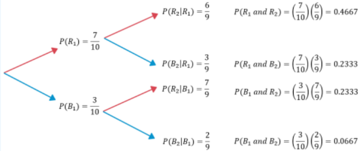
Drawing a red marble on the first draw and drawing a red marble on the second draw are dependent events because we do not place the marble back in the bag. The probability of drawing a red marble on the first draw is P(R1) = \(\frac{7}{10}\), but on the second draw, the probability of drawing a red marble given that a red marble was drawn on the first draw is P(R2|R1) = \(\frac{6}{9}\).
Thus, by the general multiplication rule, P(R1 and R2) = P(R1)·P(R2|R1) = ( \(\frac{7}{10}\) ) ( \(\frac{6}{9}\) ) = 0.4667.
A bag contains 10 colored marbles: 7 red and 3 blue. A random experiment consists of drawing a marble from the bag, then drawing another marble without replacement. Create the tree diagram for this experiment and compute the probabilities of each outcome.
Solution

Figure 4-15
If we were to multiply the probabilities as we move from left to right up each set of tree branches as shown in Figure 4-15, we get the intersections. For example, by the general multiplication rule, P(R1 and R2) = P(R1)·P(R2|R1) = ( \(\frac{7}{10}\) ) ( \(\frac{6}{9}\) ) = 0.4667.
Put the four intersection values into a contingency table and total the rows and columns. The table will help solve probability questions of other events.
| R2 | B2 | Total | |
|---|---|---|---|
| R1 | 0.4667 | 0.2333 | 0.7 |
| B1 | 0.2333 | 0.0667 | 0.3 |
| Total | 0.7 | 0.3 | 1 |
The grand total should add up to 1 since we have 100% of the sample space.
Conditional Probability Rule: P (A |B ) = \(\frac{P(A \cap B)}{P(B)}\) or P (B |A ) = \(\frac{P(A \cap B)}{P(A)}\)
The following table shows the utility contract granted for a specific year. One contractor is randomly chosen.
A random sample of 500 people was taken from the 2010 United States Census. Their marital status and race were recorded in the following contingency table. A person is randomly chosen, find the following.
Keep in mind that P(A | B) ≠ P(B | A) since we would divide by a different total in the equation.
A blood test correctly detects a certain disease 95% of the time (positive result), and correctly detects no disease present 90% of the time (negative result). It is estimated that 25% of the population have the disease. A person takes the blood test and they get a positive result. What is the probability that they have the disease?
Solution
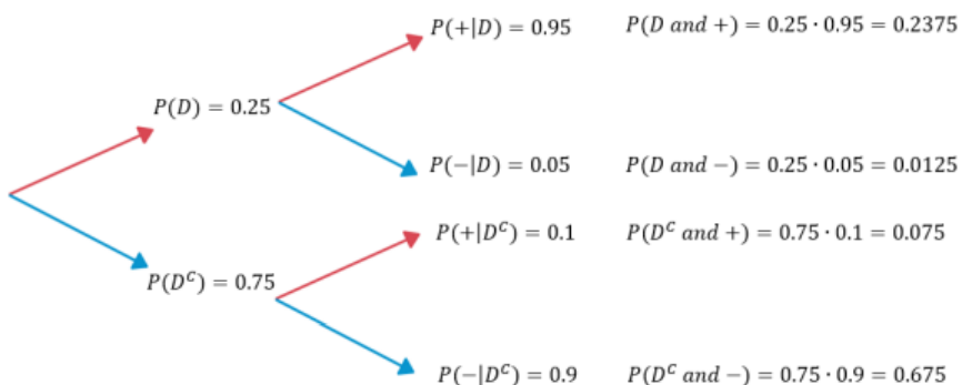
Let D = Having the Disease, DC = Not having the disease, + is a positive result, and – is a negative result. We are given in the problem the following: P(+ | D) = 0.95, P(– | DC ) = 0.90, P(D) = 0.25. We want to find P (D|+) = \(\frac{P(D \cap+)}{P(+)}\).

Figure 4-16
When you multiply up each pair of tree branches from left to right as shown in Figure 4-16, you are finding the intersection of the events. Place the multiplied values into a table. Note that the 0.2375 is not our answer. This is the people who have the disease and tested positive, but does not take into consideration the false positives. Since we know that the result was positive, we only divide by the proportion of positive results.
| DC | D | Total | |
|---|---|---|---|
| + | 0.075 | 0.2375 | 0.3125 |
| – | 0.675 | 0.0125 | 0.6875 |
| Total | 0.75 | 0.25 | 1 |
\[P (D|+) = \frac{P(D \cap+)}{P(+)} = \frac{0.2375}{0.3125} = 0.76\]
There is a 76% chance that they have the disease given that they tested positive. Many of the more difficult probability problems can be set up in a table, which makes the probabilities easier to find.


