13.2: Example Calculations
- Page ID
- 2160
\( \newcommand{\vecs}[1]{\overset { \scriptstyle \rightharpoonup} {\mathbf{#1}} } \)
\( \newcommand{\vecd}[1]{\overset{-\!-\!\rightharpoonup}{\vphantom{a}\smash {#1}}} \)
\( \newcommand{\dsum}{\displaystyle\sum\limits} \)
\( \newcommand{\dint}{\displaystyle\int\limits} \)
\( \newcommand{\dlim}{\displaystyle\lim\limits} \)
\( \newcommand{\id}{\mathrm{id}}\) \( \newcommand{\Span}{\mathrm{span}}\)
( \newcommand{\kernel}{\mathrm{null}\,}\) \( \newcommand{\range}{\mathrm{range}\,}\)
\( \newcommand{\RealPart}{\mathrm{Re}}\) \( \newcommand{\ImaginaryPart}{\mathrm{Im}}\)
\( \newcommand{\Argument}{\mathrm{Arg}}\) \( \newcommand{\norm}[1]{\| #1 \|}\)
\( \newcommand{\inner}[2]{\langle #1, #2 \rangle}\)
\( \newcommand{\Span}{\mathrm{span}}\)
\( \newcommand{\id}{\mathrm{id}}\)
\( \newcommand{\Span}{\mathrm{span}}\)
\( \newcommand{\kernel}{\mathrm{null}\,}\)
\( \newcommand{\range}{\mathrm{range}\,}\)
\( \newcommand{\RealPart}{\mathrm{Re}}\)
\( \newcommand{\ImaginaryPart}{\mathrm{Im}}\)
\( \newcommand{\Argument}{\mathrm{Arg}}\)
\( \newcommand{\norm}[1]{\| #1 \|}\)
\( \newcommand{\inner}[2]{\langle #1, #2 \rangle}\)
\( \newcommand{\Span}{\mathrm{span}}\) \( \newcommand{\AA}{\unicode[.8,0]{x212B}}\)
\( \newcommand{\vectorA}[1]{\vec{#1}} % arrow\)
\( \newcommand{\vectorAt}[1]{\vec{\text{#1}}} % arrow\)
\( \newcommand{\vectorB}[1]{\overset { \scriptstyle \rightharpoonup} {\mathbf{#1}} } \)
\( \newcommand{\vectorC}[1]{\textbf{#1}} \)
\( \newcommand{\vectorD}[1]{\overrightarrow{#1}} \)
\( \newcommand{\vectorDt}[1]{\overrightarrow{\text{#1}}} \)
\( \newcommand{\vectE}[1]{\overset{-\!-\!\rightharpoonup}{\vphantom{a}\smash{\mathbf {#1}}}} \)
\( \newcommand{\vecs}[1]{\overset { \scriptstyle \rightharpoonup} {\mathbf{#1}} } \)
\(\newcommand{\longvect}{\overrightarrow}\)
\( \newcommand{\vecd}[1]{\overset{-\!-\!\rightharpoonup}{\vphantom{a}\smash {#1}}} \)
\(\newcommand{\avec}{\mathbf a}\) \(\newcommand{\bvec}{\mathbf b}\) \(\newcommand{\cvec}{\mathbf c}\) \(\newcommand{\dvec}{\mathbf d}\) \(\newcommand{\dtil}{\widetilde{\mathbf d}}\) \(\newcommand{\evec}{\mathbf e}\) \(\newcommand{\fvec}{\mathbf f}\) \(\newcommand{\nvec}{\mathbf n}\) \(\newcommand{\pvec}{\mathbf p}\) \(\newcommand{\qvec}{\mathbf q}\) \(\newcommand{\svec}{\mathbf s}\) \(\newcommand{\tvec}{\mathbf t}\) \(\newcommand{\uvec}{\mathbf u}\) \(\newcommand{\vvec}{\mathbf v}\) \(\newcommand{\wvec}{\mathbf w}\) \(\newcommand{\xvec}{\mathbf x}\) \(\newcommand{\yvec}{\mathbf y}\) \(\newcommand{\zvec}{\mathbf z}\) \(\newcommand{\rvec}{\mathbf r}\) \(\newcommand{\mvec}{\mathbf m}\) \(\newcommand{\zerovec}{\mathbf 0}\) \(\newcommand{\onevec}{\mathbf 1}\) \(\newcommand{\real}{\mathbb R}\) \(\newcommand{\twovec}[2]{\left[\begin{array}{r}#1 \\ #2 \end{array}\right]}\) \(\newcommand{\ctwovec}[2]{\left[\begin{array}{c}#1 \\ #2 \end{array}\right]}\) \(\newcommand{\threevec}[3]{\left[\begin{array}{r}#1 \\ #2 \\ #3 \end{array}\right]}\) \(\newcommand{\cthreevec}[3]{\left[\begin{array}{c}#1 \\ #2 \\ #3 \end{array}\right]}\) \(\newcommand{\fourvec}[4]{\left[\begin{array}{r}#1 \\ #2 \\ #3 \\ #4 \end{array}\right]}\) \(\newcommand{\cfourvec}[4]{\left[\begin{array}{c}#1 \\ #2 \\ #3 \\ #4 \end{array}\right]}\) \(\newcommand{\fivevec}[5]{\left[\begin{array}{r}#1 \\ #2 \\ #3 \\ #4 \\ #5 \\ \end{array}\right]}\) \(\newcommand{\cfivevec}[5]{\left[\begin{array}{c}#1 \\ #2 \\ #3 \\ #4 \\ #5 \\ \end{array}\right]}\) \(\newcommand{\mattwo}[4]{\left[\begin{array}{rr}#1 \amp #2 \\ #3 \amp #4 \\ \end{array}\right]}\) \(\newcommand{\laspan}[1]{\text{Span}\{#1\}}\) \(\newcommand{\bcal}{\cal B}\) \(\newcommand{\ccal}{\cal C}\) \(\newcommand{\scal}{\cal S}\) \(\newcommand{\wcal}{\cal W}\) \(\newcommand{\ecal}{\cal E}\) \(\newcommand{\coords}[2]{\left\{#1\right\}_{#2}}\) \(\newcommand{\gray}[1]{\color{gray}{#1}}\) \(\newcommand{\lgray}[1]{\color{lightgray}{#1}}\) \(\newcommand{\rank}{\operatorname{rank}}\) \(\newcommand{\row}{\text{Row}}\) \(\newcommand{\col}{\text{Col}}\) \(\renewcommand{\row}{\text{Row}}\) \(\newcommand{\nul}{\text{Nul}}\) \(\newcommand{\var}{\text{Var}}\) \(\newcommand{\corr}{\text{corr}}\) \(\newcommand{\len}[1]{\left|#1\right|}\) \(\newcommand{\bbar}{\overline{\bvec}}\) \(\newcommand{\bhat}{\widehat{\bvec}}\) \(\newcommand{\bperp}{\bvec^\perp}\) \(\newcommand{\xhat}{\widehat{\xvec}}\) \(\newcommand{\vhat}{\widehat{\vvec}}\) \(\newcommand{\uhat}{\widehat{\uvec}}\) \(\newcommand{\what}{\widehat{\wvec}}\) \(\newcommand{\Sighat}{\widehat{\Sigma}}\) \(\newcommand{\lt}{<}\) \(\newcommand{\gt}{>}\) \(\newcommand{\amp}{&}\) \(\definecolor{fillinmathshade}{gray}{0.9}\)skills to develop
- Compute power using the binomial distribution
- Compute power using the normal distribution
- Use a power calculator to compute power for the \(t\) distribution
In the "Shaking and Stirring Martinis" case study, the question was whether Mr. Bond could tell the difference between martinis that were stirred and martinis that were shaken. For the sake of this example, assume he can tell the difference and is able to correctly state whether a martini had been shaken or stirred \(0.75\) of the time. Now, suppose an experiment is being conducted to investigate whether Mr. Bond can tell the difference. Specifically, is Mr. Bond correct more than \(0.50\) of the time? We know that he is (that's an assumption of the example). However, the experimenter does not know and asks Mr. Bond to judge \(16\) martinis. The experimenter will do a significance test based on the binomial distribution. Specifically, if a one tailed test is significant at the \(0.05\) level, then he or she will conclude that Mr. Bond can tell the difference. The probability value is computed assuming the null hypothesis is true (\(\pi =0.50\)). Therefore, the experimenter will determine how many times Mr. Bond is correct, and compute the probability of being correct that many or more times given that the null hypothesis is true. The question is: what is the probability the experimenter will correctly reject the null hypothesis that \(\pi =0.50\)? In other words, what is the power of this experiment?
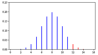
The binomial distribution for \(N = 16\) and \(\pi =0.50\) is shown in Figure \(\PageIndex{1}\). The probability of being correct on \(11\) or more trials is \(0.105\) and the probability of being correct on \(12\) or more trials is \(0.038\). Therefore, the probability of being correct on \(12\) or more trials is less than \(0.05\). This means that the null hypothesis will be rejected if Mr. Bond is correct on \(12\) or more trials and will not be rejected otherwise.
Binomial Calculator

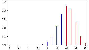
We know that Mr. Bond is correct \(0.75\) of the time. (Obviously the experimenter does not know this or there would be no need for an experiment.) The binomial distribution with \(N = 16\) and \(\pi =0.75\) is shown in Figure \(\PageIndex{2}\).

The probability of being correct on \(12\) or more trials is \(0.63\). Therefore, the power of the experiment is \(0.63\).
To sum up, the probability of being correct on \(12\) or more trials given that the null hypothesis is true is less than \(0.05\). Therefore, if Mr. Bond is correct on \(12\) or more trials, the null hypothesis will be rejected. Given Mr. Bond's true ability to be correct on \(0.75\) of the trials, the probability he will be correct on \(12\) or more trials is \(0.63\). Therefore power is \(0.63\).
In the section on Testing a Single Mean for significance, the first example was based on the assumption that the experimenter knew the population variance. Although this is rarely true in practice, the example is very useful for pedagogical purposes. For the same reason, the following example assumes the experimenter knows the population variance. Power calculators are available for situations in which the experimenter does not know the population variance.
Suppose a math achievement test were known to have a mean of \(75\) and a standard deviation of \(10\). A researcher is interested in whether a new method of teaching results in a higher mean. Assume that although the experimenter does not know it, the population mean for the new method is \(80\). The researcher plans to sample \(25\) subjects and do a one-tailed test of whether the sample mean is significantly higher than \(75\). What is the probability that the researcher will correctly reject the false null hypothesis that the population mean for the new method is \(75\) or lower? The following shows how this probability is computed.
The researcher assumes that the population standard deviation with the new method is the same as with the old method (\(10\)) and that the distribution is normal. Since the population standard deviation is assumed to be known, the researcher can use the normal distribution rather than the t distribution to compute the \(p\) value. Recall that the standard error of the mean (\(\sigma _M\)) is
\[\sigma _M=\frac{\sigma }{\sqrt{N}}\]
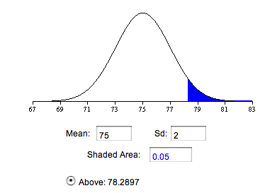
which is equal to \(10/5 = 2\) in this example. As can be seen in Figure \(\PageIndex{3}\), if the null hypothesis that the population mean equals \(75\) is true, then the probability of a sample mean being greater than or equal to \(78.29\) is \(0.05\). Therefore, the experimenter will reject the null hypothesis if the sample mean, \(M\), is \(78.29\) or larger.

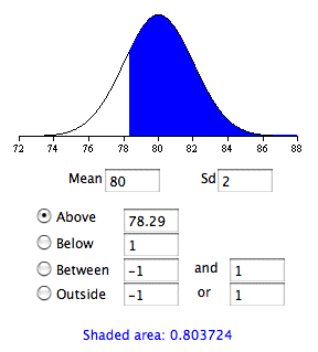
The question, then, is what is the probability the experimenter gets a sample mean greater than \(78.29\) given that the population mean is \(80\)? Figure \(\PageIndex{4}\)shows that this probability is \(0.80\).

Therefore, the probability that the experimenter will reject the null hypothesis that the population mean of the new method is \(75\) is \(0.80\). In other words, \(power = 0.80\).
Calculation of power is more complex for \(t\) tests and for Analysis of Variance. The power calculator computes power for a \(t\) test of independent groups. Calculators for other types of designs are linked to below:
Russ Lenth's Power Calculators


