
Answers to most problems


- Last updated
- Jan 11, 2021
- Save as PDF

( \newcommand{\kernel}{\mathrm{null}\,}\)
Answers are provided for most problems so you can immediately check your answers to see if you are doing it correctly. This should facilitate learning. Answers are not provided for some problems to simulate real-world conditions and tests, since answers are not known in either case.
Chapter 1
1a. parameter
1b. statistic
2. parameter
4a. H0:μ=20 H1:μ>20
4c. H0:μA=μC H1:μA≠μC
4d. H0:pm=pA H1:pm≠pA
6.
| p-value | α | Hypothesis H0 or H1 | Significant or Not Significant | Error Type I or Type II |
| 0.043 | 0.05 | H1 | Significant | Type I |
| 0.32 | 0.05 | H0 | Not Significant | Type II |
| 5.6×10⁻⁶ | 0.05 | H1 | Significant | Type I |
| 7.3256 | 0.01 | x | x | x |
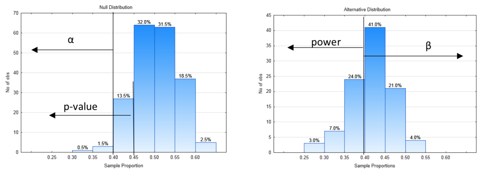
7a. At the 5% level of significance, the proportion is significantly greater than 0.5 (p = 0.022, n = 350).
7b. At the 1% level of significance, the proportion is not significantly less than 0.25 (p = 0.048, n = 1400).
7d. At the 5% level of significance, the mean is different than 20 (5.6×10⁻⁵, n = 32).
8.
8a. Left
8c. 0.40
8e. 0.66
8h. 0.155
8i. H0
8j. No
8k. type II
8l. At the 2% level of significance, the proportion is not significantly less than 0.5 (p = 0.155, n = 80).
9.
9a. Right
9c. 340
9d. 0.035
9f. 0.67
9h. 0.005
9i. H1
9j. Yes
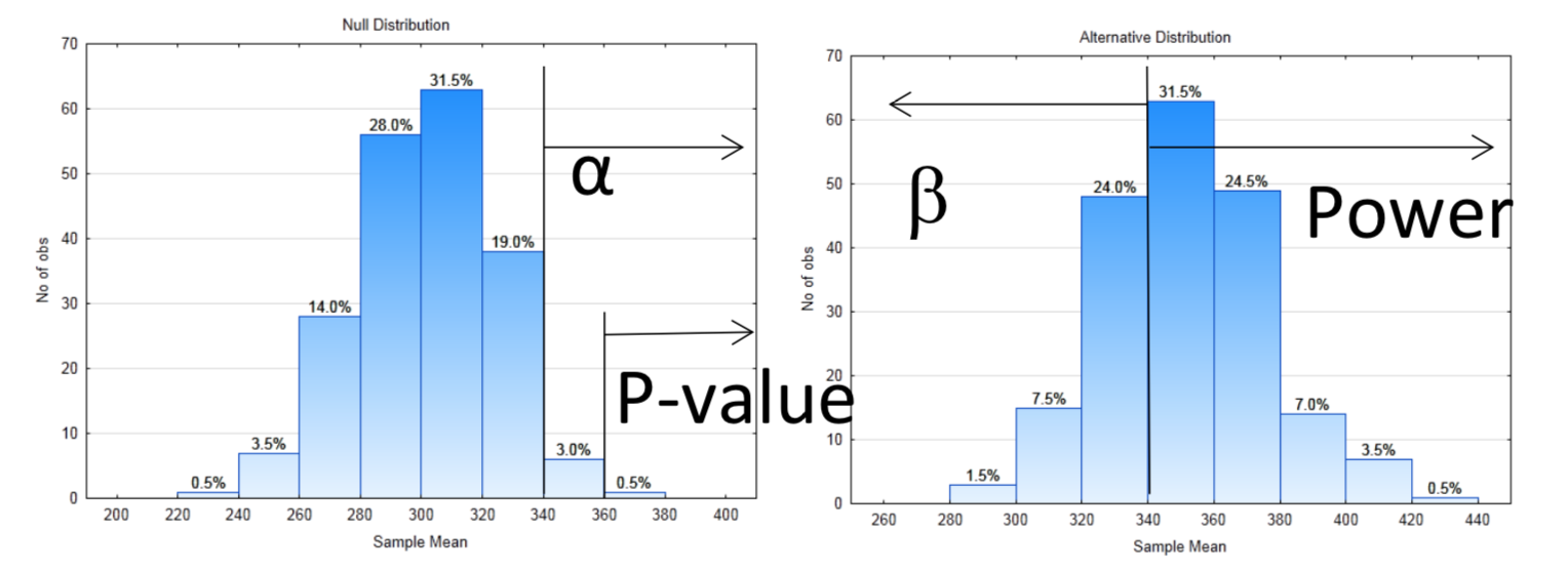
9l. At the 0.035 level of significance, the mean is significantly greater than 300 (p = 0.005, n = 10).
10a. H0:p=0.5 H1:p>0.5
10b. Right
10d. 60
10f. 0.56
10g. 0.44
10h. 0
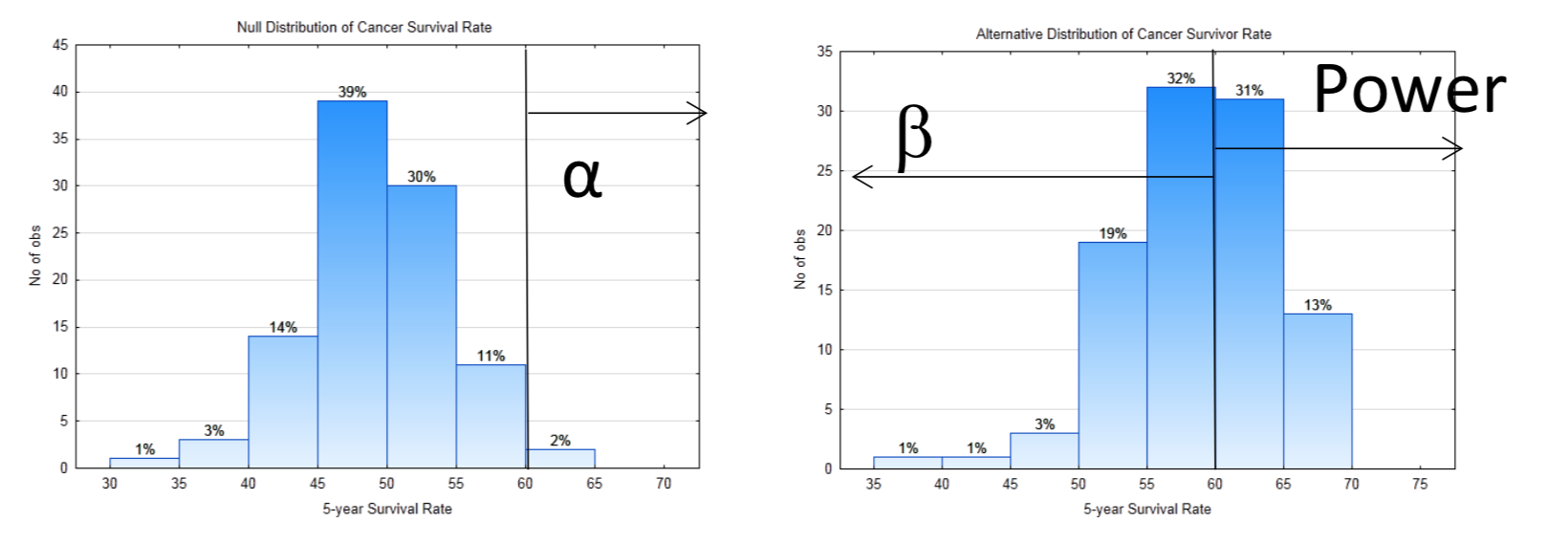
10i. At the 2% level of significance, the proportion who survive cancer at least 5 years is significantly greater than 0.5 (p = 0, n = 100).
Chapter 2
1.
| Research Design Table | |
| Research Question: which route has a faster average time | |
| Type of Research | Observational Study Observational Experiment Manipulative Experiment |
| What is the response variable? | Time it takes for the commute |
| What is the parameter that will be calculated? | Mean Proportion Correlation |
| List potential latent variables | Think of at least 2 yourself |
|
Grouping/explanatory Variables 1 (if present) routes |
Levels: Route 1 and Route 2 |
3.
| Research Design Table | |
| Research Question: Which is more effective at increasing biodiversity, the hands-off approach or the deliberate approach? | |
| Type of Research | Observational Study Observational Experiment Manipulative Experiment |
| What is the response variable? | Number of species |
| What is the parameter that will be calculated? | Mean Proportion Correlation |
| List potential latent variables | Think of at least 2 yourself |
|
Grouping/explanatory Variables 1 (if present) approaches |
Levels: hands-off deliberate control |
4b.
| Research Design Table | |
| Research Question: Does static or dynamic stretching result in improvement in flexibility in the largest proportion of people? | |
| Type of Research | Observational Study Observational Experiment Manipulative Experiment |
| What is the response variable? | Improvement in sit and reach test |
| What is the parameter that will be calculated? | Mean Proportion |
| List potential latent variables | Think of at least 2 yourself |
|
Grouping/explanatory Variables 1 (if present) Stretching method |
Levels: static dynamic |
8a. 102 N, 40 N, 18 Y, 49 N, 61 N, 60 N, 57 N, 16 N, 90 N, 46 Y,
135 N, 105 Y, 83 N, 102 N, 3 N, 70 Y, 47 N, 42 N, 5 N, 68 N,
Sample Proportion __4/20 = 0.2
8b. West 37 Y,45 N, 21 N, 56 N, 70 Y, 68 N, 65 N, 18 Y, 22 N, 52 Y, 75 Y,
East 93 N, 105 Y, 109 N, 90 N, 114 N, 137 Y, 133 N, 131 N, 104 Y
Sample Proportion _8/20 = 0.4
8c. 2 Y, 9 N, 16 N, 23 N, 30 N, 37 Y, 44 Y, 51 Y, 58 N, 65 N,
72 Y, 79 N, 86 Y, 93 N, 100 N, 107 N, 114 N, 121 N, 128 N, 135 N,
Sample Proportion _6/20 = .30
8d. Which cluster is selected? ___7____ Sample Proportion _9/20=0.45
8m 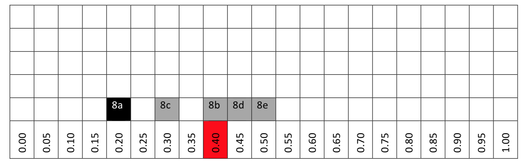
9a.
| Research Design Table | |
| Research Question: Does raising the minimum wage cause unemployment to increase? | |
| Type of Research | Observational Study Observational Experiment Manipulative Experiment |
| What is the response variable? | Change in Unemployment rate |
| What is the parameter that will be calculated? | Mean Proportion Correlation |
| List potential latent variables | Think of at least 2 yourself |
|
Grouping/explanatory Variables 1 (if present) State minimum wage change |
Levels: Increase minimum wage No change in minimum wage |
9b. Cluster
9c. 2004, 2012, 2006
9d. Provide your own thoughtful answer.
9e. Provide your own thoughtful answer.
9f. Provide your own thoughtful answer.
9g. At the 5% level of significance, there is not a significant difference in the change in unemployment rate between states that raised their minimum wage and those that didn’t (p = 0.286).
10a.
| Research Design Table | |
| Research Question: Will the number of falls increase after bedrails are removed? | |
| Type of Research | Observational Study Observational Experiment Manipulative Experiment |
| What is the response variable? | Falls |
| What is the parameter that will be calculated? | Mean Proportion Correlation |
| List potential latent variables | Think of at least 2 yourself |
|
Grouping/explanatory Variables 1 (if present) Bedrails |
Levels: Present |
10b. At the 5% level of significance, there was not a significant increase in the number of falls per 10,000 bed days after the implementation of the new policy (p = 0.18).
10c. There were fewer serious falls, more minor and no-injury falls. A possible reason is that the falls are from a lower height since the patient isn’t crawling over the top of the rails.
10d. Provide your own thoughtful response.
Chapter 3
1.
2.
3. mean = 43, Standard deviation = 4.78, variance = 22.89
4.
5. r=cov(x,y)sxsy=2.095.56⋅1.20=0.313
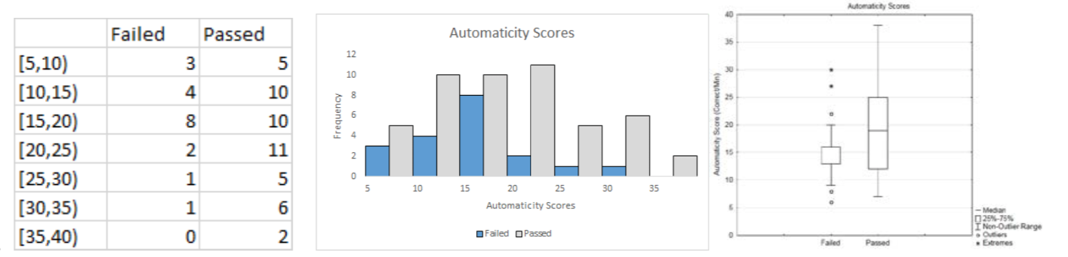
6a.
| Research Design Table | |
| Research Question: Is average number of problems answered correctly in one minute was greater for students who passed the class than for those who didn’t pass? | |
| Type of Research | Observational Study Observational Experiment Manipulative Experiment |
| What is the response variable? | Number of correctly answered problems |
| What is the parameter that will be calculated? | Mean Proportion Correlation |
| List potential latent variables | |
|
Grouping/explanatory Variables 1 (if present) Success in course |
Levels: Pass Fail |
| Grouping/explanatory Variables 2 (if present) | Levels: |
6b. Calc: 2,9
6c. Cluster
6d. Quantitative discrete
6e.
6f. Provide your own thoughtful response.
6g.
| Mean | Variance | Standard Deviation | |
| Failed | 15.89 | 33.88 | 5.82 |
| Passed |
6h. At the 5% level of significance, the average automaticity score of those who pass the class is significantly more than the score of those who fail the class (p = 0.0395, nfail = 19, npass = 49).
6i. Yes
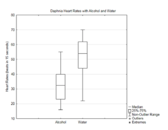
7a.
| Research Design Table | |
| Research Question: Is the average heart rate lower with alcohol than with water? | |
| Type of Research | Observational Study Observational Experiment Manipulative Experiment |
| What is the response variable? | heart rate |
| What is the parameter that will be calculated? | Mean Proportion Correlation |
| List potential latent variables | List you own ideas |
|
Grouping/explanatory Variables 1 (if present) drop |
Levels: water (first time) alcohol, water (second time) |
| Grouping/explanatory Variables 2 (if present) | Levels: |
7b.
7c.
| Heart Rate after Alcohol | Heart Rate after Water | |
| mean | 32.8 | 52.1 |
| Standard Deviation | 10.7 | 13.0 |
| Median | 32.5 | 54.0 |
7d. At the 5% level of significance, the average daphnia heart rate with alcohol is significantly less than the average daphnia heart rate with water (p = 1.28×10⁻⁵, nalcohol = 18, nwater = 18).
7e. Provide your own thoughtful answer.
Chapter 4
1.
1a. P(S) = 0.70
1b. P(F) = 0.30
1c. P(FSSSF) = P(F)P(S) P(S) P(S) P(F) = (0.3) (0.7) (0.7) (0.7) (0.3) = 0.03087
1d. 10
1e. 0.3087
1f.
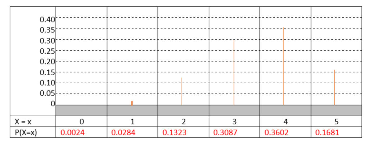
1g. μ=np=5(0.7)=3.5 σ=√npq=√5(0.7)(0.3)=1.025
1h. P(X≤3) = binomcdf(n, p, x) = binomcdf (5, 0.70, 3) = 0.4718. The null is supported. The data are not significant.
2.
2a. P(S) = 0.40
2b. P(F) = 0.60
2c. 0.0036864
2d. 21
2e. 0.0774
2f.
| X=x | 0 | 1 | 2 | 3 | 4 | 5 | 6 | 7 |
| P(X=x) | 0.0280 | 0.1306 | 0.2613 | 0.2903 | 0.1935 | 0.0774 | 0.0172 | 0.0016 |
2g. 2.8, 1.296
2h. P-value = 0.0963 alternative
3.
3j. P-value = 0.047
At the 5% level of significance, the proportion of residents opposed to the terminals is significantly greater than 0.5 (p = 0.047, n = 300)
3k. z = 1.73 p-value 0.0418
At the 5% level of significance, the proportion of residents opposed to the terminals is significantly greater than 0.5 (z = 1.73, p = 0.0418, n = 300).
3l. 0.55
3m. 0.02887
3n. z = 1.73 p-value 0.0418
At the 5% level of significance, the proportion of residents opposed to the terminals is significantly greater than 0.5 (z = 1.73, p = 0.0418, n = 300).
4a. H0:μ=43,362 and H1:μ<43,362
4b. μ=43,362
4c. σˉx=σ√n=7900√10=2498
4d.
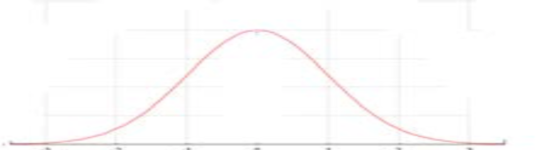
X axis: 35868 38366 40864 43362 45860 48358 50856
4e. 18,225 (use stat-edit and then stat-calc-1-var stats)
4f. z = -10.06 p-value < 0.0002
6b. H0:μ=54.1 and H1:μ>54.1
6d. barx=46.73, s=16.377
6e. μ=54.1 σˉx=2.939
6f.
45.4 48.3 51.2 54.1 57 59.9 62.8
6g. z = -2.51 p-value 0.9940
At the 5% level of significance, the average walk score of small cities is not significantly greater than big cities (z = -2.51, p = 0.994, n = 30)
7e. p-value = 0.3865 0.0148
7g p-value = 0.0129
7h z = 2.229, p= 0.0129
8c.
| Impact | Control | |
| Mean | 455 | |
| Standard Deviation | 614.8 | |
| Median | 150 |
Chapter 5
1a. H0:μT=μD H1:μT≠μD Test: 2 independent samples t test
1b. H0:p=0.5 H1:p>0.5 Test: 1 proportion z test
1c. H0:pSTEM=pSS H1:pSTEM≠pSS Test: 2 proportion Z test
1e. H0:μ=7 H1:μ>7 Test: 1 sample t test
1g. H0:μ=0 H1:μ<0 Test: 1 sample t test
2a. H0:μ=15, H1:μ<15
2b. Test the bypothesis:
t=ˉx−μs√n t=14.28−154.6√30 t = -0.857 p > 0.1 or p = 0.1991
Formula Substitution Test Statistic p-value
2c. Fill in the blanks for the concluding sentence. At the _5%__ level of significance, the mean money spent per day _is not_ significantly less than $15 (t = ____________, p ___________, df = 29).
3a. Write the hypotheses: H0:p=0.5, H1:p>0.5, Sample proportion (ˆp) = 118179 = 0.659
3b. Test the hypothesis:
z=ˆp−p√p(1−pn z=0.659−0.5√0.5(1−0.5179 p < 0.0002 or 1.02 ×10⁻⁵
Formula Substitution Test Statistic p-value
Write the concluding sentence: At the 5% level of significance, the average price on Tuesday is not significantly less than other days (t = -0.479, p > 0.25, n = 7).
5a. Write the hypotheses: H0: _ μ40=μ60 ___, H1: __μ40<μ60__,
5c. Write the concluding sentence: At the 10% level of significance, the mean guess at Morocco’s population by people with low phone digits is significantly less than the mean guess of those with high phone digits (t = -1.835, p < 0.05, n40 = 15, n60 = 15).
6c. Test the hypothesis: Test Statistic = -12.41, p-value = p =1
7e. Write a concluding sentence. At the 5% level of significance, the proportion of 12th grade students using drugs in 2012 is not significantly greater than in 2002 (z = 0.819, p = 0.2061, n2012 = 630, n2002 = 2184).
8a.
| Research Design Table | |
| Research Question: Is there a significant difference in the mean times of the men and women who finish the triathlon course? | |
| Type of Research | Observational Study Observational Experiment Manipulative Experiment |
| What is the response variable? | heart rate |
| What is the parameter that will be calculated? | Mean Proportion Correlation |
| List potential confounding variables | |
|
Grouping/explanatory Variables 1 (if present) Gender |
Levels: Men, Women |
8b. Write the hypotheses. H0:μmen=μwomen, H1:μmen≠μwomen
9a. Conclusion: At the 5% level of significance, there is not a significant difference in the proportion of days that African Americans and LGB individuals record at least one stigma-related stressor (z = 0.062, p=0.950, nAA = 190, nLGB = 310)
9b. Conclusion: At the 5% level of significance, the mean psychological distress score for those using rumination is significantly different than for those using distraction (t = 2.189, p = 0.033, nR = 26, nD = 26)
Chapter 6
1. 0.778
Margin of Error 0.060 Confidence Interval (0.718,0.838) Calculator confidence interval (0.71853,0.83823)
2. Girls: 0.743, Boys 0.778
Margin of Error 0.132, Confidence Interval (9-0.167,0.097)
3. (Note: There are 112 degrees of freedom. This df does not appear in your tables. It falls between 60 df and 120 df. To make sure that the interval is sufficiently large, the critical t value for 60 df will be used. The actual value, as found using the Excel function T.INV.2T(0.1,112) is 1.6586).
Margin of error 14.6 (73.4,102.6)
Calculator confidence interval (73.49,102.51)
5. Point estimate 156
Margin of error 92.9 Confidence Interval (63.1,248.9)
Calculator confidence interval (63.087,248.91)
6. Point Estimate 5.2 degrees
Margin of error 3.2 confidence interval (2,8.4)
Calculator confidence interval (2.0338,8.3662)
8. Point estimate 0.116
Margin of Error 0.017, Confidence interval (0.099,0.133)
9.
| Margin of Error | 1% | 5% | 10% | 20% |
| Sample Size | 9604 |
10.
| Degree of Confidence | 99% | 95% | 90% | 80% |
| Sample Size | 1844 |
11a. Stratified
11b. 256 , 379 ,
11d. Mean = 59.5, SD = 23.78
11e. (48.4, 70.6)
11f. Lowest: 290.4
Chapter 7
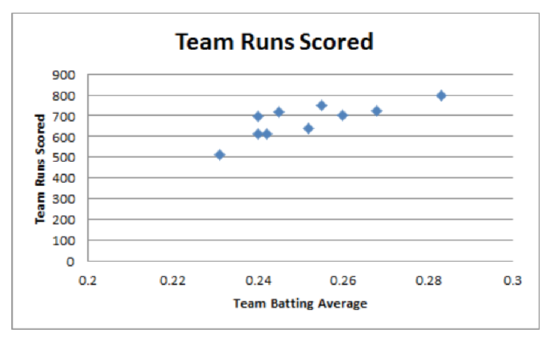
1b Mean batting average 0.2516 Standard deviation for batting average 0.0155
Mean runs scored 676.1 Standard deviation for runs scored 82.20
1c. At the 5% level of significance, there is a significant correlation between batting average and runs scored (t = 3.84, p < 0.01, n = 10).
1d. Regression equation: y = -397.98 + 4269x
1e. r2 = 0.6479. It means 64.8% of the total variation from the mean for team runs scored is attributed to the variation in the batting average.
1f. 669.285
1g.
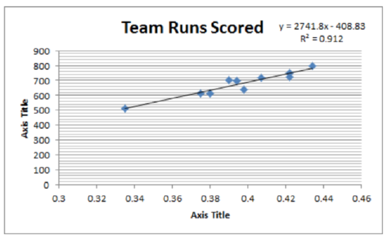
Correlation: 0.955
Hypothesis test concluding sentence: At the 5% level of significance, there is a significant correlation between slugging percentage and runs scored (t = 9.10, p = 1.699E-5, n = 10).
Regression equation: y=−408.83+2741.80x
Coefficient of determination (r2): 0.912
Predict the number of runs scored for a team with a slugging percentage of 0.400. 687.89
2a.
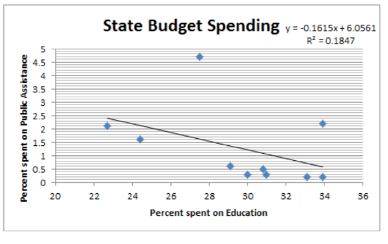
2b.
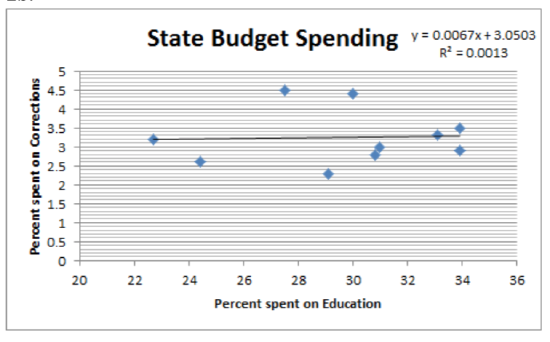
R = 0.0359, r2 = 0.0013, y=3.05+0.0067x
At the 5% level of significance, there is not a significant correlation between spending on education and spending on public assistance (t = -1.35, p = 0.215, n = 10).
3.
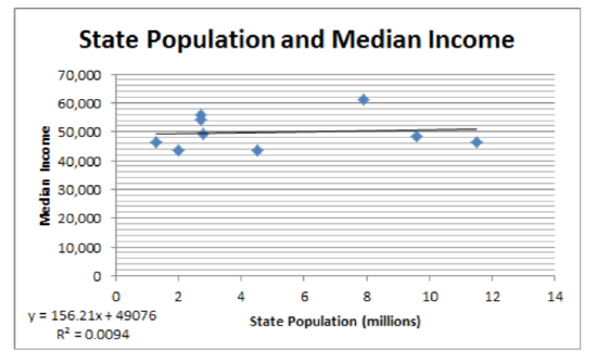
Y=49075.6+156.2x r=0.097, r2=0.0094, t=0.258, p=0.8038.
4a.
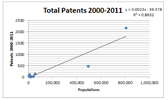
Y=−36.38+0.0023x r=0.929, r2=0.863, t=6.64, p=2.92×10⁻⁴
4b. Provide your own thoughtful response.
4c. 101.62
5a. Age
5b. NPA
5c. 2, 12, 22, 32, 42, 52, 62, 72, 82, 92, 102
5e. r = 0.814
5f. At the 5% level of significance, there is a significant correlation between age and NPA (t = 4.2, p = 0.002, n = 11).
Chapter 8
1a. Test for Homogeneity
1b. Goodness of Fit
1c. Test for Independence
1d. Goodness of Fit
2.
| X=x | 0 | 1 | 2 | 3 |
| P(X=x) | 0.5787 | 0.34722 | 0.06944 | 0.00463 |
Goodness of Fit
χ2=3.43
At the 5% level of significance, there is not a significant difference between the observed and expected distributions (χ2=3.43, p>0.1, n=158) . Calculator p-value is 0.33.
3. Test for Independence
χ2 = 13.27
At the 0.1 level of significance there is a correlation between shots and goals (χ2=13.27, p<0.005, n=49) (calculator p-value = 2.696×10⁻⁴).
4. Test for Homogeneity
At the 0.1 level of significance, the distributions for improvement from drug and non-drug treatments are homogeneous (χ2=0.8222, p>0.1, n=80) (Calculator: p=0.6629, df=2)
5. χ2=9.426
6a. stratified
6b. 2042, 584, _____
6c. Goodness of Fit
6d.
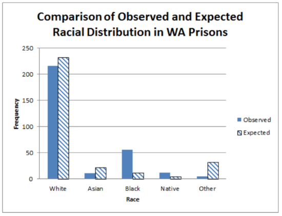
6f. At the 5% level of significance, the racial distribution of WA prisons is significantly different than what would be expected (χ2=229.96, p<0.005, n=300) (Calculator: p=1.3×10−48, df = 4).