10.8: New Models for One Population Inference, Similar Procedures

Last updated
Save as PDF

Page ID: 20911

\( \newcommand{\vecs}[1]{\overset { \scriptstyle \rightharpoonup} {\mathbf{#1}} } \) \( \newcommand{\vecd}[1]{\overset{-\!-\!\rightharpoonup}{\vphantom{a}\smash {#1}}} \)\(\newcommand{\id}{\mathrm{id}}\) \( \newcommand{\Span}{\mathrm{span}}\) \( \newcommand{\kernel}{\mathrm{null}\,}\) \( \newcommand{\range}{\mathrm{range}\,}\) \( \newcommand{\RealPart}{\mathrm{Re}}\) \( \newcommand{\ImaginaryPart}{\mathrm{Im}}\) \( \newcommand{\Argument}{\mathrm{Arg}}\) \( \newcommand{\norm}[1]{\| #1 \|}\) \( \newcommand{\inner}[2]{\langle #1, #2 \rangle}\) \( \newcommand{\Span}{\mathrm{span}}\) \(\newcommand{\id}{\mathrm{id}}\) \( \newcommand{\Span}{\mathrm{span}}\) \( \newcommand{\kernel}{\mathrm{null}\,}\) \( \newcommand{\range}{\mathrm{range}\,}\) \( \newcommand{\RealPart}{\mathrm{Re}}\) \( \newcommand{\ImaginaryPart}{\mathrm{Im}}\) \( \newcommand{\Argument}{\mathrm{Arg}}\) \( \newcommand{\norm}[1]{\| #1 \|}\) \( \newcommand{\inner}[2]{\langle #1, #2 \rangle}\) \( \newcommand{\Span}{\mathrm{span}}\)\(\newcommand{\AA}{\unicode[.8,0]{x212B}}\)

The procedures outlined for the test of population mean vs. hypothesized value with known population standard deviation will apply to other models as well. All that really changes is the test statistic.

Examples of some other one population models:

Test of population mean vs. hypothesized value, population standard deviation unknown.
Test of population proportion vs. hypothesized value.
Test of population standard deviation (or variance) vs. hypothesized value.

Test of population mean with unknown population standard deviation

The test statistic for the one sample case changes to a Student’s t distribution with degrees of freedom equal to \(n-1: t=\dfrac{\overline{X}-\mu_{o}}{s / \sqrt{n}}\)

The shape of the \(t\) distribution is similar to the \(Z\), except for the fact that the tails are fatter, so the logic of the decision rule is the same as for the \(Z\) test statistic.

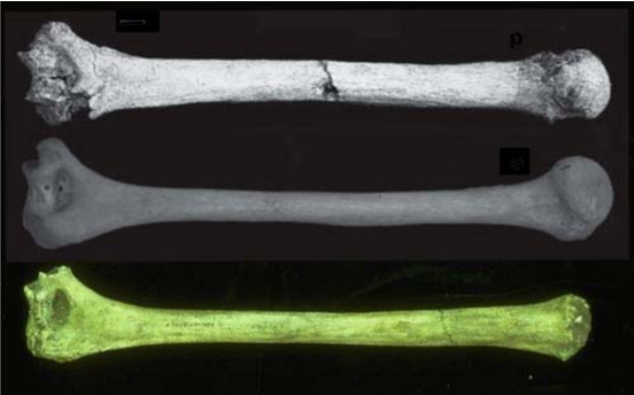
Example: Archaeology

Humerus bones from the same species have approximately the same length‐to‐width ratios. When fossils of humerus bones are discovered, archaeologists can determine the species by examining this ratio. It is known that Species A has a mean ratio of 9.6. A similar Species B has a mean ratio of 9.1 and is often confused with Species A. 21 humerus bones were unearthed in an area that was originally thought to be inhabited Species A. (Assume all unearthed bones are from the same species.)

Design a test in which the alternative hypothesis would be the humerus bones were not from Species A.
Determine the power of this test if the bones actually came from Species B (assume a standard deviation of 0.7)
Conduct the test using at a 5% significance level and state overall conclusions.

Solution

Research Hypotheses

\(H_o: \mu=9.6\) (The humerus bones are from Species A)

\(H_a: \mu\neq9.6\) (The humerus bones are not from Species A)

Significance level: \(\alpha\) =.05

Test Statistic (Model): \(t\)‐test of mean vs. hypothesized value, unknown standard deviation

Model Assumptions: we may need to check the data for extreme skewness as the distribution of the sample mean is assumed to be approximately the Normal Distribution.

Information needed for Power Calculation	Results using Online Power Calculator⁷⁵
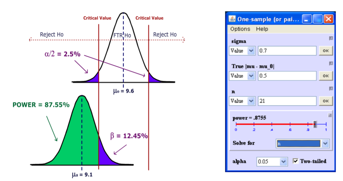
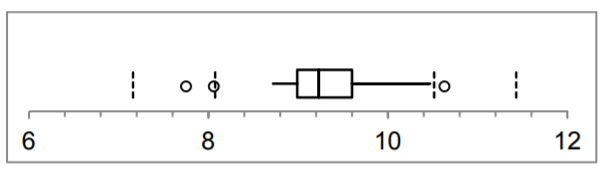
\(\mu_{o}\) = 9.6 (Species A) \(\mu_{a}\) = 9.1 (Species B) Effect Size =\(\| mo ‐ ma \|\) = 0.5 \(s\) = 0.7 (given) \(\alpha\) = .05 \(n\) = 21 (sample size) Two tailed test	Power =.8755 \(\beta\) = 1 ‐ Power = .1245 If humerus bones are from Species B, test has an 87.55% chance of correctly rejecting Ho and a maximum Type II error of 12.55%

From MegaStat⁷⁶, \(p\)‐value = .0308 and \(\alpha\) =.05.

Since \(p\)‐value < \(\alpha\), \(H_o\) is rejected and we support \(H_a\).

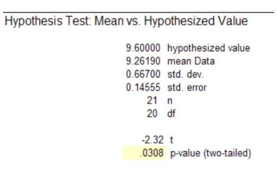
Conclusion: The evidence supports the claim (\(p\)‐value < .05) that the humerus bones are not from Species A. The small sample size limited the power of the test, which prevented us from making a more definitive conclusion. Further testing is recommended to determine if bones are from Species B or other unknown species.

We are also assuming that since the bones were unearthed in the same location, they came from the same species.

Test of population proportion vs. hypothesized value

When our data is categorical and there are only two possible choices (for example a yes/no question on a poll), we may want to make a claim about a proportion or a percentage of the population (\(p\)) being compared to a particular value (\(p_o\)). We will then use the sample proportion (\(\hat{p}\)) to test the claim.

Test of proportion vs. hypothesized value

\(p\) = population proportion

\(p_o\) = population proportion under \(H_o\)

\(\hat{p}\) = sample proportion

\(p_a\) = population proportion under Ha

Test Statistic: \(Z=\dfrac{\hat{p}-p_{o}}{\sqrt{\frac{p_{o}\left(1-p_{o}\right)}{n}}}\)

Requirement for Normality Assumption: \(n p(1-p)>5\)

Example: Charity solicitation

In the past, 15% of the mail order solicitations for a certain charity resulted in a financial contribution. A new solicitation letter has been drafted and will be sent to a random sample of potential donors. A hypothesis test will be run to determine if the new letter is more effective. Determine the sample so that (1) the test will be run at the 5% significance level and (2) if the letter has an 18% success rate, (an effect size of 3%), the power of the test will be 95%. After determining the sample size, conduct the test.

Solution

\(H_o: p \leq 0.15\) (The new letter is not more effective.)

\(H_a: p > 0.15\) (The new letter is more effective.)

Test Statistic – \(Z\)‐test of proportion vs. hypothesized value

Information needed for Power Calculation	Results using Online Power Calculator⁷⁵
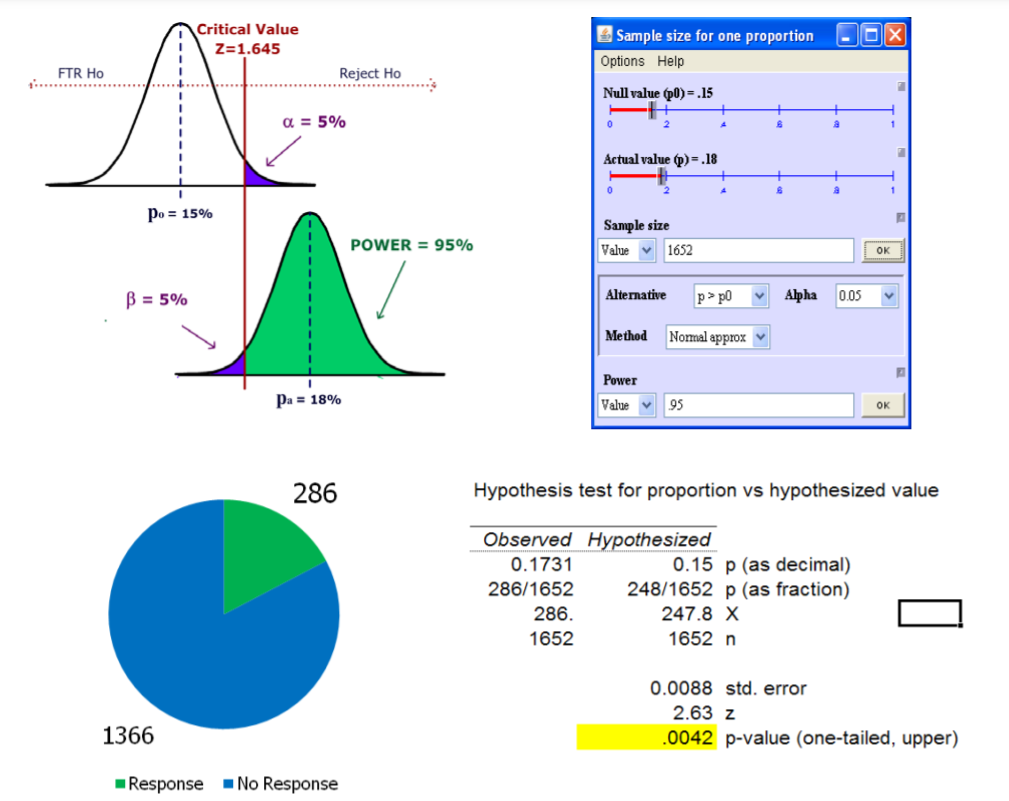
\(p_{o}\) = 0.15 (current letter) \(p_{a}\) = 0.18 (potential new letter) Effect Size = \(\| pa ‐ po \|\) = 0.03 Desired Power = 0.95 \(\alpha\) = .05 One tailed test	Sample size = 1652 The charity sent out 1652 new solicitation letters to potential donors and ran the test, receiving 286 positive responses. \(p\)‐value for test = 0.0042

Since \(p\)‐value < \(\alpha\), reject \(H_o\) and support \(H_a\). Since the \(p\)‐value is actually less than 0.01, we would go further and say that the data supports rejecting \(H_o\) for \(\alpha = .01\).

Conclusion: The evidence supports the claim that the new letter is more effective. The 1652 test letters were selected as a random sample from the charity’s mailing list. All letters were sent at the same time period. The letters needed to be sent in a specific time period, so we were not able to control for seasonal or economic factors. We recommend testing both solicitation methods over the entire year to eliminate seasonal effects and to create a control group.

Test of population standard deviation (or variance) vs. hypothesized value

We often want to make a claim about the variability, volatility or consistency of a population random variable. Hypothesized values for the population variance (\(\sigma^{2}\)) or the standard deviation (\(\sigma\)) are tested with the Chi‐square (\(\chi^{2}\)) distribution.

Examples of Hypotheses:

\(H_o: \sigma = 10 \) \(H_a: \sigma \neq 10\)
\(H_o: \sigma^{2} = 100\) \(H_a: \sigma^{2} > 100\)

The sample variance \(s^2\) is used in calculating the Chi‐square Test Statistic.

Test of variance vs. hypothesized value

\(\sigma^{2}\) = population variance

\(\sigma_{o}^{2}\) = population variance under Ho

\(s^2\) = sample variance

Test Statistic: \(\chi^{2}=\dfrac{(n-1) s^{2}}{\sigma_{o}^{2}}\)

\(n-1\) = degrees of freedom

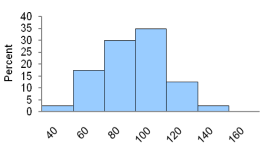
Example: Standardized testing

A state school administrator claims that the standard deviation of test scores for 8^th grade students who took a life‐science assessment test is less than 30, meaning the results for the class show consistency. An auditor wants to support that claim by analyzing 41 students’ recent test scores. The test will be run at 1% significance level.

\(\begin{array}{|l|l|l|l|l|l|l|l|l|}
\hline 57 & 75 & 86 & 92 & 101 & 108 & 110 & 120 & 155 \\
\hline 63 & 77 & 88 & 96 & 102 & 108 & 111 & 122 & \\
\hline 66 & 78 & 88 & 96 & 107 & 109 & 115 & 135 & \\
\hline 68 & 81 & 92 & 98 & 107 & 109 & 115 & 137 & \\
\hline 72 & 82 & 92 & 99 & 107 & 110 & 118 & 139 & \\
\hline
\end{array}\)

Solution

Design:

Research Hypotheses:

\(H_o\): Standard deviation for test scores equals 30.

\(H_a\): Standard deviation for test scores is less than 30.

Hypotheses In terms of the population variance:

\(H_o: \sigma^{2} = 900\)

\(H_a: \sigma^{2} < 900\)

Results:

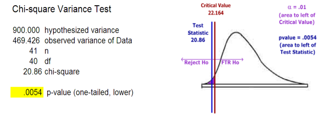
Decision: Reject \(H_o\)

Conclusion: The evidence supports the claim (\(p\)‐value < .01) that the standard deviation for 8^th grade test scores is less than 30. The 40 test scores were the results of the recently administered exam to the 8^th grade students. Since the exams were for the current class only, there is no assurance that future classes will achieve similar results. Further research would be to compare results to other schools that administered the same exam and to continue to analyze future class exams to see if the claim is holding true.