10.7: Type II Error and Statistical Power

In the prior example, the statistician failed to reject the Null Hypothesis because the probability of making Type I error (rejecting a true Null Hypothesis) exceeded the significance level of 5%. However, the statistician could have made Type II error if the machine is really operating improperly. One of the important and often overlooked tasks is to analyze the probability of making Type II error (\(\beta\)). Usually statisticians look at statistical power which is the complement of \(\beta\).

 

Beta (\(\beta\)): The probability of failing to reject the null hypothesis when it is actually false.

Power (or Statistical Power): The probability of rejecting  the null hypothesis when it is actually false.

Both beta and power are calculated for specific possible values of the Alternative Hypothesis.

	Fail to Reject \(H_o\)	Reject \(H_o\)
\(H_o\) is true	\(1-\alpha\)	\(\alpha\) Type I error
\(H_o\) is false	\(\beta\) Type II error	\(1-\beta\) Power

If a hypothesis test has low power, then it would be difficult to reject \(H_o\), even if \(H_o\) were false; the research would be a waste of time and money. However, analyzing power is difficult in that there are many values of the population parameter that support \(H_a\). For example, in the soy sauce bottling example, the Alternative Hypothesis was that the mean was not 16 ounces. This means the machine could be filling the bottles with a mean of 16.0001 ounces, making Ha technically true. So when analyzing power and Type II error, we need to choose a value for the population mean under the Alternative Hypothesis (\(\mu_a\)) that is “practically different” from the mean under the Null Hypothesis (\(\mu_o\)). This practical difference is called the effect size.

Definition: Effect size

Effect Size: The “practical difference” between \(\mu_{o}\) and \(\mu_a=\left|\mu_{o}-\mu_{a}\right|\)

where 

\(\mu_{o}\): The value of the population mean under the Null Hypothesis

\(\mu_{a}\): The value of the population mean under the Alternative Hypothesis

Suppose we are conducting a one‐tailed test of the population mean:  

\[H_o: \mu=\mu_{0} \qquad Ha: \mu>\mu_{0} \nonumber \]

Consider the two graphs shown below. The top graph is the distribution of the sample mean under the Null Hypothesis, which was covered in an earlier section. The area to the right of the critical value is the rejection region.

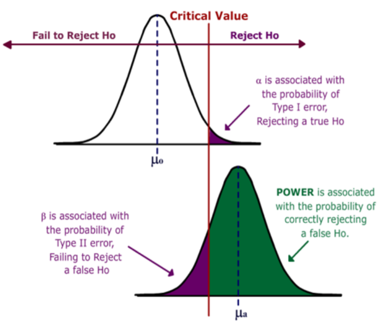
We now add the bottom graph, which represents the distribution of the sample mean under the Alternative Hypothesis for the specific value \(\mu a\).

We can now measure the Power of the test (the area in green) and beta (the area in purple) on the lower graph.  

There are several methods of increasing Power, but they all have trade‐offs:

Ways to Increase Power	Trade off
Increase Sample Size	Increased cost or unavailability of data
Increase Significance level (\(\alpha\))	More like to Reject a true \(H_o\) (Type I error)
Choose a value of \(\mu_{a}\) further from \(\mu_{o}\)	Result may be less meaningful
Redefine population to lower standard deviation	Result may be too limited to have value
Conduct as a one‐tail rather than a two‐tail test	May produce a biased result

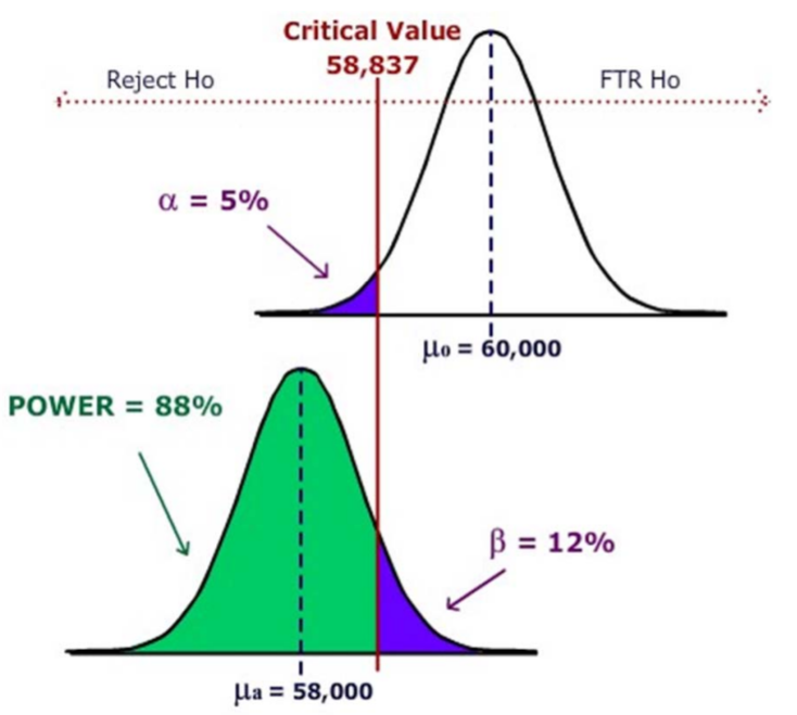
Example: Bus brake pads

Bus brake pads are claimed to last on average at least 60,000 miles and the company wants to test this claim. The bus company considers a “practical” value for purposes of bus safety to be that the pads last at least 58,000 miles. If the standard deviation is 5,000 and the sample size is 50, find the power of the test when the mean is really 58,000 miles. (Assume \(\alpha = .05\)) 

Solution

First, find the critical value of the test.

Reject \(H_o\) when \(Z < ‐1.645\)

Next,  find the value of that corresponds to the critical value.

\[\overline{X}=\mu_{o}+\dfrac{Z \sigma}{\sqrt{n}}=60000-(1.645)(5000) / \sqrt{50}=58837 \nonumber \]

\(H_o\) is rejected when \(\overline{X}<58837\)

Finally, find the probability of rejecting \(H_o\) if Ha is true.

\[\begin{aligned}
P(\overline{X}<58837) &=P\left(Z<\dfrac{\left(58837-\mu_{a}\right)}{\sigma / \sqrt{n}}\right) \\
&=P\left(Z<\dfrac{(58837-58000)}{5000 / \sqrt{50}}\right)\\
&=P(Z<1.18)\\
&=.8810
\end{aligned} \nonumber \]

Therefore, this test has 88% power and \(\beta\) would be 12%

Power Calculation Values

Input Values

\(\mu_{o}\) = 60,000 miles

\(\mu_{a}\) = 58,000 miles

\(\alpha\) = 0.05 ݊

\(n\) = 50

\(\sigma\) = 5000 miles

Calculated Values

Effect Size = 2000 miles

Critical Value = 58,837 miles

\(\beta\) = 0.1190 or about 12%

Power = 0.8810 or about 88%