3.3: Hypothesis Test about the Population Mean when the Population Standard Deviation is Unknown
- Page ID
- 2885
\( \newcommand{\vecs}[1]{\overset { \scriptstyle \rightharpoonup} {\mathbf{#1}} } \)
\( \newcommand{\vecd}[1]{\overset{-\!-\!\rightharpoonup}{\vphantom{a}\smash {#1}}} \)
\( \newcommand{\id}{\mathrm{id}}\) \( \newcommand{\Span}{\mathrm{span}}\)
( \newcommand{\kernel}{\mathrm{null}\,}\) \( \newcommand{\range}{\mathrm{range}\,}\)
\( \newcommand{\RealPart}{\mathrm{Re}}\) \( \newcommand{\ImaginaryPart}{\mathrm{Im}}\)
\( \newcommand{\Argument}{\mathrm{Arg}}\) \( \newcommand{\norm}[1]{\| #1 \|}\)
\( \newcommand{\inner}[2]{\langle #1, #2 \rangle}\)
\( \newcommand{\Span}{\mathrm{span}}\)
\( \newcommand{\id}{\mathrm{id}}\)
\( \newcommand{\Span}{\mathrm{span}}\)
\( \newcommand{\kernel}{\mathrm{null}\,}\)
\( \newcommand{\range}{\mathrm{range}\,}\)
\( \newcommand{\RealPart}{\mathrm{Re}}\)
\( \newcommand{\ImaginaryPart}{\mathrm{Im}}\)
\( \newcommand{\Argument}{\mathrm{Arg}}\)
\( \newcommand{\norm}[1]{\| #1 \|}\)
\( \newcommand{\inner}[2]{\langle #1, #2 \rangle}\)
\( \newcommand{\Span}{\mathrm{span}}\) \( \newcommand{\AA}{\unicode[.8,0]{x212B}}\)
\( \newcommand{\vectorA}[1]{\vec{#1}} % arrow\)
\( \newcommand{\vectorAt}[1]{\vec{\text{#1}}} % arrow\)
\( \newcommand{\vectorB}[1]{\overset { \scriptstyle \rightharpoonup} {\mathbf{#1}} } \)
\( \newcommand{\vectorC}[1]{\textbf{#1}} \)
\( \newcommand{\vectorD}[1]{\overrightarrow{#1}} \)
\( \newcommand{\vectorDt}[1]{\overrightarrow{\text{#1}}} \)
\( \newcommand{\vectE}[1]{\overset{-\!-\!\rightharpoonup}{\vphantom{a}\smash{\mathbf {#1}}}} \)
\( \newcommand{\vecs}[1]{\overset { \scriptstyle \rightharpoonup} {\mathbf{#1}} } \)
\( \newcommand{\vecd}[1]{\overset{-\!-\!\rightharpoonup}{\vphantom{a}\smash {#1}}} \)
\(\newcommand{\avec}{\mathbf a}\) \(\newcommand{\bvec}{\mathbf b}\) \(\newcommand{\cvec}{\mathbf c}\) \(\newcommand{\dvec}{\mathbf d}\) \(\newcommand{\dtil}{\widetilde{\mathbf d}}\) \(\newcommand{\evec}{\mathbf e}\) \(\newcommand{\fvec}{\mathbf f}\) \(\newcommand{\nvec}{\mathbf n}\) \(\newcommand{\pvec}{\mathbf p}\) \(\newcommand{\qvec}{\mathbf q}\) \(\newcommand{\svec}{\mathbf s}\) \(\newcommand{\tvec}{\mathbf t}\) \(\newcommand{\uvec}{\mathbf u}\) \(\newcommand{\vvec}{\mathbf v}\) \(\newcommand{\wvec}{\mathbf w}\) \(\newcommand{\xvec}{\mathbf x}\) \(\newcommand{\yvec}{\mathbf y}\) \(\newcommand{\zvec}{\mathbf z}\) \(\newcommand{\rvec}{\mathbf r}\) \(\newcommand{\mvec}{\mathbf m}\) \(\newcommand{\zerovec}{\mathbf 0}\) \(\newcommand{\onevec}{\mathbf 1}\) \(\newcommand{\real}{\mathbb R}\) \(\newcommand{\twovec}[2]{\left[\begin{array}{r}#1 \\ #2 \end{array}\right]}\) \(\newcommand{\ctwovec}[2]{\left[\begin{array}{c}#1 \\ #2 \end{array}\right]}\) \(\newcommand{\threevec}[3]{\left[\begin{array}{r}#1 \\ #2 \\ #3 \end{array}\right]}\) \(\newcommand{\cthreevec}[3]{\left[\begin{array}{c}#1 \\ #2 \\ #3 \end{array}\right]}\) \(\newcommand{\fourvec}[4]{\left[\begin{array}{r}#1 \\ #2 \\ #3 \\ #4 \end{array}\right]}\) \(\newcommand{\cfourvec}[4]{\left[\begin{array}{c}#1 \\ #2 \\ #3 \\ #4 \end{array}\right]}\) \(\newcommand{\fivevec}[5]{\left[\begin{array}{r}#1 \\ #2 \\ #3 \\ #4 \\ #5 \\ \end{array}\right]}\) \(\newcommand{\cfivevec}[5]{\left[\begin{array}{c}#1 \\ #2 \\ #3 \\ #4 \\ #5 \\ \end{array}\right]}\) \(\newcommand{\mattwo}[4]{\left[\begin{array}{rr}#1 \amp #2 \\ #3 \amp #4 \\ \end{array}\right]}\) \(\newcommand{\laspan}[1]{\text{Span}\{#1\}}\) \(\newcommand{\bcal}{\cal B}\) \(\newcommand{\ccal}{\cal C}\) \(\newcommand{\scal}{\cal S}\) \(\newcommand{\wcal}{\cal W}\) \(\newcommand{\ecal}{\cal E}\) \(\newcommand{\coords}[2]{\left\{#1\right\}_{#2}}\) \(\newcommand{\gray}[1]{\color{gray}{#1}}\) \(\newcommand{\lgray}[1]{\color{lightgray}{#1}}\) \(\newcommand{\rank}{\operatorname{rank}}\) \(\newcommand{\row}{\text{Row}}\) \(\newcommand{\col}{\text{Col}}\) \(\renewcommand{\row}{\text{Row}}\) \(\newcommand{\nul}{\text{Nul}}\) \(\newcommand{\var}{\text{Var}}\) \(\newcommand{\corr}{\text{corr}}\) \(\newcommand{\len}[1]{\left|#1\right|}\) \(\newcommand{\bbar}{\overline{\bvec}}\) \(\newcommand{\bhat}{\widehat{\bvec}}\) \(\newcommand{\bperp}{\bvec^\perp}\) \(\newcommand{\xhat}{\widehat{\xvec}}\) \(\newcommand{\vhat}{\widehat{\vvec}}\) \(\newcommand{\uhat}{\widehat{\uvec}}\) \(\newcommand{\what}{\widehat{\wvec}}\) \(\newcommand{\Sighat}{\widehat{\Sigma}}\) \(\newcommand{\lt}{<}\) \(\newcommand{\gt}{>}\) \(\newcommand{\amp}{&}\) \(\definecolor{fillinmathshade}{gray}{0.9}\)Hypothesis Test about the Population Mean (μ) when the Population Standard Deviation (σ) is Unknown
Frequently, the population standard deviation (σ) is not known. We can estimate the population standard deviation (σ) with the sample standard deviation (s). However, the test statistic will no longer follow the standard normal distribution. We must rely on the student’s t-distribution with n-1 degrees of freedom. Because we use the sample standard deviation (s), the test statistic will change from a Z-score to a t-score.
\[z=\frac {\bar {x}-\mu}{\frac {\sigma}{\sqrt {n}}} \longrightarrow t = \frac {\bar {x} - \mu}{\frac {s}{\sqrt {n}}}\]
Steps for a hypothesis test are the same that we covered in Section 2.
- State the null and alternative hypotheses.
- State the level of significance and the critical value.
- Compute the test statistic.
- State a conclusion.
Just as with the hypothesis test from the previous section, the data for this test must be from a random sample and requires either that the population from which the sample was drawn be normal or that the sample size is sufficiently large (n≥30). A t-test is robust, so small departures from normality will not adversely affect the results of the test. That being said, if the sample size is smaller than 30, it is always good to verify the assumption of normality through a normal probability plot.
We will still have the same three pairs of null and alternative hypotheses and we can still use either the classical approach or the p-value approach.
Table \(PageIndex{1}\): The rejection zone for a two-sided hypothesis test.
|
Two-sided |
Left-sided |
Right-sided |
|---|---|---|
|
\(\mathrm{H}_{\mathrm{O}}: \boldsymbol{\mu}=\mathrm{c}\) |
\(\mathbf{H}_{\mathbf{0}}: \boldsymbol{\mu}=\mathbf{C}\) |
\(\mathbf{H}_{\mathbf{0}}: \boldsymbol{\mu}=\mathbf{C}\) |
|
\(\mathbf{H}_{\mathbf{1}}: \boldsymbol{\mu \neq \mathbf { C }}\) |
\(\mathbf{H}_{\mathbf{1}}: \boldsymbol{\mu}< \mathbf{C}\) |
\(\mathbf{H}_{\mathbf{1}}: \boldsymbol{\mu}>\mathbf{C}\) |
Selecting the correct critical value from the student’s t-distribution table depends on three factors: the type of test (one-sided or two-sided alternative hypothesis), the sample size, and the level of significance.
For a two-sided test (“not equal” alternative hypothesis), the critical value (tα/2), is determined by alpha (α), the level of significance, divided by two, to deal with the possibility that the result could be less than OR greater than the known value.
- If your level of significance was 0.05, you would use the 0.025 column to find the correct critical value (0.05/2 = 0.025).
- If your level of significance was 0.01, you would use the 0.005 column to find the correct critical value (0.01/2 = 0.005).
For a one-sided test (“a less than” or “greater than” alternative hypothesis), the critical value (tα) , is determined by alpha (α), the level of significance, being all in the one side.
- If your level of significance was 0.05, you would use the 0.05 column to find the correct critical value for either a left or right-side question. If you are asking a “less than” (left-sided question, your critical value will be negative. If you are asking a “greater than” (right-sided question), your critical value will be positive.
Find the critical value you would use to test the claim that μ ≠ 112 with a sample size of 18 and a 5% level of significance.
Solution
In this case, the critical value (\(t_{α/2}\)) would be 2.110. This is a two-sided question (≠) so you would divide alpha by 2 (0.05/2 = 0.025) and go down the 0.025 column to 17 degrees of freedom.
What would the critical value be if you wanted to test that μ < 112 for the same data?
Solution
In this case, the critical value would be 1.740. This is a one-sided question (<) so alpha would be divided by 1 (0.05/1 = 0.05). You would go down the 0.05 column with 17 degrees of freedom to get the correct critical value.
In 2005, the mean pH level of rain in a county in northern New York was 5.41. A biologist believes that the rain acidity has changed. He takes a random sample of 11 rain dates in 2010 and obtains the following data. Use a 1% level of significance to test his claim.
4.70, 5.63, 5.02, 5.78, 4.99, 5.91, 5.76, 5.54, 5.25, 5.18, 5.01
The sample size is small and we don’t know anything about the distribution of the population, so we examine a normal probability plot. The distribution looks normal so we will continue with our test.
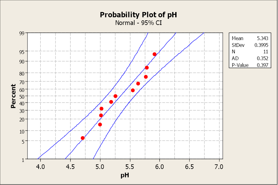
The sample mean is 5.343 with a sample standard deviation of 0.397.
Solution
Step 1) State the null and alternative hypotheses.
- Ho: μ = 5.41
- H1: μ ≠ 5.41
Step 2) State the level of significance and the critical value.
- This is a two-sided question so alpha is divided by two.
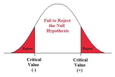
Figure \(\PageIndex{2}\): The rejection zones for a two-sided test.
- t α/2 is found by going down the 0.005 column with 14 degrees of freedom.
- t α/2 = ±3.169.
Step 3) Compute the test statistic.
- The test statistic is a t-score.
\[t=\frac {\bar {x}-\mu}{\frac {s}{sqrt {n}}}\]
- For this problem, the test statistic is
\[t=\frac {5.343-5.41}{\frac {0.397}{\sqrt {11}}} = -0.560 \nonumber \]
Step 4) State a conclusion.
- Compare the test statistic to the critical value.
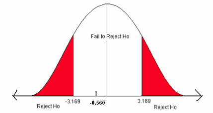
Figure \(\PageIndex{3}\): The critical values for a two-sided test when α = 0.01.
- The test statistic does not fall in the rejection zone.
We will fail to reject the null hypothesis. We do not have enough evidence to support the claim that the mean rain pH has changed.
Cadmium, a heavy metal, is toxic to animals. Mushrooms, however, are able to absorb and accumulate cadmium at high concentrations. The government has set safety limits for cadmium in dry vegetables at 0.5 ppm. Biologists believe that the mean level of cadmium in mushrooms growing near strip mines is greater than the recommended limit of 0.5 ppm, negatively impacting the animals that live in this ecosystem. A random sample of 51 mushrooms gave a sample mean of 0.59 ppm with a sample standard deviation of 0.29 ppm. Use a 5% level of significance to test the claim that the mean cadmium level is greater than the acceptable limit of 0.5 ppm.
The sample size is greater than 30 so we are assured of a normal distribution of the means.
Solution
Step 1) State the null and alternative hypotheses.
- Ho: μ = 0.5 ppm
- H1: μ > 0.5 ppm
Step 2) State the level of significance and the critical value.
- This is a right-sided question so alpha is all in the right tail.
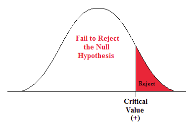
Figure \(\PageIndex{4}\): Rejection zone for a right-sided test.
- t α is found by going down the 0.05 column with 50 degrees of freedom.
- t α = 1.676
Step 3) Compute the test statistic.
- The test statistic is a t-score.
\[t=\frac {\bar {x}-\mu}{\frac {s}{\sqrt {n}}}\]
- For this problem, the test statistic is
\[t=\frac {0.59-0.50}{\frac {0.29}{\sqrt {51}}}=2.216 \nonumber \]
Step 4) State a Conclusion.
- Compare the test statistic to the critical value.
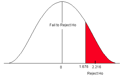
Figure \(\PageIndex{5}\): Critical value for a right-sided test when α = 0.05.
The test statistic falls in the rejection zone. We will reject the null hypothesis. We have enough evidence to support the claim that the mean cadmium level is greater than the acceptable safe limit.
BUT, what happens if the significance level changes to 1%?
The critical value is now found by going down the 0.01 column with 50 degrees of freedom. The critical value is 2.403. The test statistic is now LESS THAN the critical value. The test statistic does not fall in the rejection zone. The conclusion will change. We do NOT have enough evidence to support the claim that the mean cadmium level is greater than the acceptable safe limit of 0.5 ppm.
The level of significance is the probability that you, as the researcher, set to decide if there is enough statistical evidence to support the alternative claim. It should be set before the experiment begins.
P-value Approach
We can also use the p-value approach for a hypothesis test about the mean when the population standard deviation (σ) is unknown. However, when using a student’s t-table, we can only estimate the range of the p-value, not a specific value as when using the standard normal table. The student’s t-table has area (probability) across the top row in the table, with t-scores in the body of the table.
- To find the p-value (the area associated with the test statistic), you would go to the row with the number of degrees of freedom.
- Go across that row until you find the two values that your test statistic is between, then go up those columns to find the estimated range for the p-value.
Estimating P-value from a Student’s T-table
Table \(PageIndex{2}\). Portion of the student’s t-table. t- distribution, Area in right tail.
|
df |
.05 |
.025 |
.02 |
.01 |
.005 |
|---|---|---|---|---|---|
|
1 |
6.314 |
12.706 |
15.894 |
31.821 |
63.657 |
|
2 |
2.920 |
4.303 |
4.849 |
6.965 |
9.925 |
|
3 |
2.353 |
3.182 |
3.482 |
4.541 |
5.841 |
|
4 |
2.132 |
2.776 |
2.999 |
3.747 |
4.604 |
|
5 |
2.015 |
2.571 |
2.757 |
3.365 |
4.032 |
Solution
If your test statistic is 3.789 with 3 degrees of freedom, you would go across the 3 df row. The value 3.789 falls between the values 3.482 and 4.541 in that row. Therefore, the p-value is between 0.02 and 0.01. The p-value will be greater than 0.01 but less than 0.02 (0.01<p<0.02).
Conclusion
If your level of significance is 5%, you would reject the null hypothesis as the p-value (0.01-0.02) is less than alpha (α) of 0.05.
If your level of significance is 1%, you would fail to reject the null hypothesis as the p-value (0.01-0.02) is greater than alpha (α) of 0.01.
Software packages typically output p-values. It is easy to use the Decision Rule to answer your research question by the p-value method.
Software Solutions
Minitab
(referring to Ex. 5)
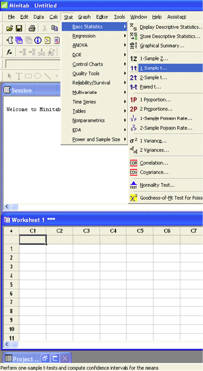
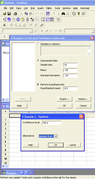
One-Sample T
Test of mu = 0.5 vs. > 0.5
95% Lower
|
N |
Mean |
StDev |
SE Mean |
Bound |
T |
P |
|
51 |
0.5900 |
0.2900 |
0.0406 |
0.5219 |
2.22 |
0.016 |
Additional example: www.youtube.com/watch?v=WwdSjO4VUsg.
Excel
Excel does not offer 1-sample hypothesis testing.


