3.2: Hypothesis Test about the Population Mean when the Population Standard Deviation is Known
- Page ID
- 2884
\( \newcommand{\vecs}[1]{\overset { \scriptstyle \rightharpoonup} {\mathbf{#1}} } \)
\( \newcommand{\vecd}[1]{\overset{-\!-\!\rightharpoonup}{\vphantom{a}\smash {#1}}} \)
\( \newcommand{\dsum}{\displaystyle\sum\limits} \)
\( \newcommand{\dint}{\displaystyle\int\limits} \)
\( \newcommand{\dlim}{\displaystyle\lim\limits} \)
\( \newcommand{\id}{\mathrm{id}}\) \( \newcommand{\Span}{\mathrm{span}}\)
( \newcommand{\kernel}{\mathrm{null}\,}\) \( \newcommand{\range}{\mathrm{range}\,}\)
\( \newcommand{\RealPart}{\mathrm{Re}}\) \( \newcommand{\ImaginaryPart}{\mathrm{Im}}\)
\( \newcommand{\Argument}{\mathrm{Arg}}\) \( \newcommand{\norm}[1]{\| #1 \|}\)
\( \newcommand{\inner}[2]{\langle #1, #2 \rangle}\)
\( \newcommand{\Span}{\mathrm{span}}\)
\( \newcommand{\id}{\mathrm{id}}\)
\( \newcommand{\Span}{\mathrm{span}}\)
\( \newcommand{\kernel}{\mathrm{null}\,}\)
\( \newcommand{\range}{\mathrm{range}\,}\)
\( \newcommand{\RealPart}{\mathrm{Re}}\)
\( \newcommand{\ImaginaryPart}{\mathrm{Im}}\)
\( \newcommand{\Argument}{\mathrm{Arg}}\)
\( \newcommand{\norm}[1]{\| #1 \|}\)
\( \newcommand{\inner}[2]{\langle #1, #2 \rangle}\)
\( \newcommand{\Span}{\mathrm{span}}\) \( \newcommand{\AA}{\unicode[.8,0]{x212B}}\)
\( \newcommand{\vectorA}[1]{\vec{#1}} % arrow\)
\( \newcommand{\vectorAt}[1]{\vec{\text{#1}}} % arrow\)
\( \newcommand{\vectorB}[1]{\overset { \scriptstyle \rightharpoonup} {\mathbf{#1}} } \)
\( \newcommand{\vectorC}[1]{\textbf{#1}} \)
\( \newcommand{\vectorD}[1]{\overrightarrow{#1}} \)
\( \newcommand{\vectorDt}[1]{\overrightarrow{\text{#1}}} \)
\( \newcommand{\vectE}[1]{\overset{-\!-\!\rightharpoonup}{\vphantom{a}\smash{\mathbf {#1}}}} \)
\( \newcommand{\vecs}[1]{\overset { \scriptstyle \rightharpoonup} {\mathbf{#1}} } \)
\(\newcommand{\longvect}{\overrightarrow}\)
\( \newcommand{\vecd}[1]{\overset{-\!-\!\rightharpoonup}{\vphantom{a}\smash {#1}}} \)
\(\newcommand{\avec}{\mathbf a}\) \(\newcommand{\bvec}{\mathbf b}\) \(\newcommand{\cvec}{\mathbf c}\) \(\newcommand{\dvec}{\mathbf d}\) \(\newcommand{\dtil}{\widetilde{\mathbf d}}\) \(\newcommand{\evec}{\mathbf e}\) \(\newcommand{\fvec}{\mathbf f}\) \(\newcommand{\nvec}{\mathbf n}\) \(\newcommand{\pvec}{\mathbf p}\) \(\newcommand{\qvec}{\mathbf q}\) \(\newcommand{\svec}{\mathbf s}\) \(\newcommand{\tvec}{\mathbf t}\) \(\newcommand{\uvec}{\mathbf u}\) \(\newcommand{\vvec}{\mathbf v}\) \(\newcommand{\wvec}{\mathbf w}\) \(\newcommand{\xvec}{\mathbf x}\) \(\newcommand{\yvec}{\mathbf y}\) \(\newcommand{\zvec}{\mathbf z}\) \(\newcommand{\rvec}{\mathbf r}\) \(\newcommand{\mvec}{\mathbf m}\) \(\newcommand{\zerovec}{\mathbf 0}\) \(\newcommand{\onevec}{\mathbf 1}\) \(\newcommand{\real}{\mathbb R}\) \(\newcommand{\twovec}[2]{\left[\begin{array}{r}#1 \\ #2 \end{array}\right]}\) \(\newcommand{\ctwovec}[2]{\left[\begin{array}{c}#1 \\ #2 \end{array}\right]}\) \(\newcommand{\threevec}[3]{\left[\begin{array}{r}#1 \\ #2 \\ #3 \end{array}\right]}\) \(\newcommand{\cthreevec}[3]{\left[\begin{array}{c}#1 \\ #2 \\ #3 \end{array}\right]}\) \(\newcommand{\fourvec}[4]{\left[\begin{array}{r}#1 \\ #2 \\ #3 \\ #4 \end{array}\right]}\) \(\newcommand{\cfourvec}[4]{\left[\begin{array}{c}#1 \\ #2 \\ #3 \\ #4 \end{array}\right]}\) \(\newcommand{\fivevec}[5]{\left[\begin{array}{r}#1 \\ #2 \\ #3 \\ #4 \\ #5 \\ \end{array}\right]}\) \(\newcommand{\cfivevec}[5]{\left[\begin{array}{c}#1 \\ #2 \\ #3 \\ #4 \\ #5 \\ \end{array}\right]}\) \(\newcommand{\mattwo}[4]{\left[\begin{array}{rr}#1 \amp #2 \\ #3 \amp #4 \\ \end{array}\right]}\) \(\newcommand{\laspan}[1]{\text{Span}\{#1\}}\) \(\newcommand{\bcal}{\cal B}\) \(\newcommand{\ccal}{\cal C}\) \(\newcommand{\scal}{\cal S}\) \(\newcommand{\wcal}{\cal W}\) \(\newcommand{\ecal}{\cal E}\) \(\newcommand{\coords}[2]{\left\{#1\right\}_{#2}}\) \(\newcommand{\gray}[1]{\color{gray}{#1}}\) \(\newcommand{\lgray}[1]{\color{lightgray}{#1}}\) \(\newcommand{\rank}{\operatorname{rank}}\) \(\newcommand{\row}{\text{Row}}\) \(\newcommand{\col}{\text{Col}}\) \(\renewcommand{\row}{\text{Row}}\) \(\newcommand{\nul}{\text{Nul}}\) \(\newcommand{\var}{\text{Var}}\) \(\newcommand{\corr}{\text{corr}}\) \(\newcommand{\len}[1]{\left|#1\right|}\) \(\newcommand{\bbar}{\overline{\bvec}}\) \(\newcommand{\bhat}{\widehat{\bvec}}\) \(\newcommand{\bperp}{\bvec^\perp}\) \(\newcommand{\xhat}{\widehat{\xvec}}\) \(\newcommand{\vhat}{\widehat{\vvec}}\) \(\newcommand{\uhat}{\widehat{\uvec}}\) \(\newcommand{\what}{\widehat{\wvec}}\) \(\newcommand{\Sighat}{\widehat{\Sigma}}\) \(\newcommand{\lt}{<}\) \(\newcommand{\gt}{>}\) \(\newcommand{\amp}{&}\) \(\definecolor{fillinmathshade}{gray}{0.9}\)Hypothesis Test about the Population Mean (μ) when the Population Standard Deviation (σ) is Known
We are going to examine two equivalent ways to perform a hypothesis test: the classical approach and the p-value approach. The classical approach is based on standard deviations. This method compares the test statistic (Z-score) to a critical value (Z-score) from the standard normal table. If the test statistic falls in the rejection zone, you reject the null hypothesis. The p-value approach is based on area under the normal curve. This method compares the area associated with the test statistic to alpha (α), the level of significance (which is also area under the normal curve). If the p-value is less than alpha, you would reject the null hypothesis.
As a past student poetically said: If the p-value is a wee value, Reject Ho
Both methods must have:
- Data from a random sample.
- Verification of the assumption of normality.
- A null and alternative hypothesis.
- A criterion that determines if we reject or fail to reject the null hypothesis.
- A conclusion that answers the question.
There are four steps required for a hypothesis test:
- State the null and alternative hypotheses.
- State the level of significance and the critical value.
- Compute the test statistic.
- State a conclusion.
The Classical Method for Testing a Claim about the Population Mean (μ) when the Population Standard Deviation (σ) is Known
A forester studying diameter growth of red pine believes that the mean diameter growth will be different from the known mean growth of 1.35 inches/year if a fertilization treatment is applied to the stand. He conducts his experiment, collects data from a sample of 32 plots, and gets a sample mean diameter growth of 1.6 in./year. The population standard deviation for this stand is known to be 0.46 in./year. Does he have enough evidence to support his claim?
Solution
Step 1) State the null and alternative hypotheses.
- Ho: μ = 1.35 in./year
- H1: μ ≠ 1.35 in./year
Step 2) State the level of significance and the critical value.
- We will choose a level of significance of 5% (α = 0.05).
- For a two-sided question, we need a two-sided critical value – Z α/2 and + Z α/2.
- The level of significance is divided by 2 (since we are only testing “not equal”). We must have two rejection zones that can deal with either a greater than or less than outcome (to the right (+) or to the left (-)).
- We need to find the Z-score associated with the area of 0.025. The red areas are equal to α/2 = 0.05/2 = 0.025 or 2.5% of the area under the normal curve.
- Go into the body of values and find the negative Z-score associated with the area 0.025.
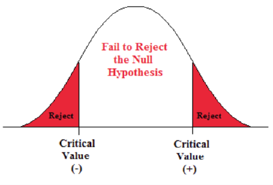
- The negative critical value is -1.96. Since the curve is symmetric, we know that the positive critical value is 1.96.
- ±1.96 are the critical values. These values set up the rejection zone. If the test statistic falls within these red rejection zones, we reject the null hypothesis.
Step 3) Compute the test statistic.
- The test statistic is the number of standard deviations the sample mean is from the known mean. It is also a Z-score, just like the critical value.
- \[z = \frac {\bar {x} -\mu}{\frac {\sigma}{\sqrt {n}}} \]
- For this problem, the test statistic is
\[z = \frac {1.6-1.35}{\frac {0.46}{\sqrt {32}}} =3.07 \nonumber \]
Step 4) State a conclusion.
- Compare the test statistic to the critical value. If the test statistic falls into the rejection zones, reject the null hypothesis. In other words, if the test statistic is greater than +1.96 or less than -1.96, reject the null hypothesis.
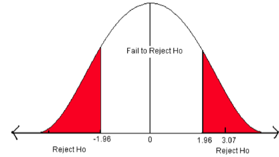
Figure \(\PageIndex{2}\): The critical values for a two-sided test when α = 0.05.
In this problem, the test statistic falls in the red rejection zone. The test statistic of 3.07 is greater than the critical value of 1.96.We will reject the null hypothesis. We have enough evidence to support the claim that the mean diameter growth is different from (not equal to) 1.35 in./year.
A researcher believes that there has been an increase in the average farm size in his state since the last study five years ago. The previous study reported a mean size of 450 acres with a population standard deviation (σ) of 167 acres. He samples 45 farms and gets a sample mean of 485.8 acres. Is there enough information to support his claim?
Solution
Step 1) State the null and alternative hypotheses.
- Ho: μ = 450 acres
- H1: μ >450 acres
Step 2) State the level of significance and the critical value.
- We will choose a level of significance of 5% (α = 0.05).
- For a one-sided question, we need a one-sided positive critical value Zα.
- The level of significance is all in the right side (the rejection zone is just on the right side).
- We need to find the Z-score associated with the 5% area in the right tail.
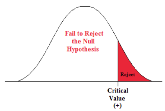
Figure \(\PageIndex{3}\): Rejection zone for a right-sided hypothesis test.
- Go into the body of values in the standard normal table and find the Z-score that separates the lower 95% from the upper 5%.
- The critical value is 1.645. This value sets up the rejection zone.
Step 3) Compute the test statistic.
- The test statistic is the number of standard deviations the sample mean is from the known mean. It is also a Z-score, just like the critical value.
- \[z = \frac {\bar {x} -\mu}{\frac {\sigma}{\sqrt {n}}}\]
- For this problem, the test statistic is
\[z = \frac {485.8-450}{\frac {167}{\sqrt {45}}} =1.44 \nonumber \]
Step 4) State a conclusion.
- Compare the test statistic to the critical value.
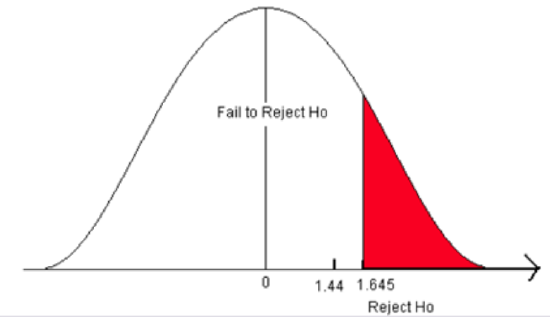
Figure \(\PageIndex{4}\): The critical value for a right-sided test when α = 0.05.
- The test statistic does not fall in the rejection zone. It is less than the critical value.
We fail to reject the null hypothesis. We do not have enough evidence to support the claim that the mean farm size has increased from 450 acres.
A researcher believes that there has been a reduction in the mean number of hours that college students spend preparing for final exams. A national study stated that students at a 4-year college spend an average of 23 hours preparing for 5 final exams each semester with a population standard deviation of 7.3 hours. The researcher sampled 227 students and found a sample mean study time of 19.6 hours. Does this indicate that the average study time for final exams has decreased? Use a 1% level of significance to test this claim.
Solution
Step 1) State the null and alternative hypotheses.
- Ho: μ = 23 hours
- H1: μ < 23 hours
Step 2) State the level of significance and the critical value.
- This is a left-sided test so alpha (0.01) is all in the left tail.
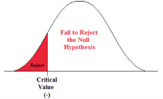
Figure \(\PageIndex{5}\): The rejection zone for a left-sided hypothesis test.
- Go into the body of values in the standard normal table and find the Z-score that defines the lower 1% of the area.
- The critical value is -2.33. This value sets up the rejection zone.
Step 3) Compute the test statistic.
- The test statistic is the number of standard deviations the sample mean is from the known mean. It is also a Z-score, just like the critical value.
- \[z = \frac {\bar {x} - \mu}{\frac {\sigma} {\sqrt {n}}}\]
- For this problem, the test statistic is
\[z= \frac {19.6-23}{\frac {7.3}{\sqrt {277}}} \nonumber \]
Step 4) State a conclusion.
- Compare the test statistic to the critical value.
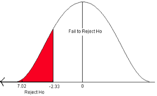
Figure \(\PageIndex{6}\): The critical value for a left-sided test when α = 0.01.
- The test statistic falls in the rejection zone. The test statistic of -7.02 is less than the critical value of -2.33.
We reject the null hypothesis. We have sufficient evidence to support the claim that the mean final exam study time has decreased below 23 hours.
Testing a Hypothesis using P-values
The p-value is the probability of observing our sample mean given that the null hypothesis is true. It is the area under the curve to the left or right of the test statistic. If the probability of observing such a sample mean is very small (less than the level of significance), we would reject the null hypothesis. Computations for the p-value depend on whether it is a one- or two-sided test.
Steps for a hypothesis test using p-values:
- State the null and alternative hypotheses.
- State the level of significance.
- Compute the test statistic and find the area associated with it (this is the p-value).
- Compare the p-value to alpha (α) and state a conclusion.
Instead of comparing Z-score test statistic to Z-score critical value, as in the classical method, we compare area of the test statistic to area of the level of significance.
If the p-value is less than alpha, we reject the null hypothesis.
Computing P-values
If it is a two-sided test (the alternative claim is ≠), the p-value is equal to two times the probability of the absolute value of the test statistic. If the test is a left-sided test (the alternative claim is “<”), then the p-value is equal to the area to the left of the test statistic. If the test is a right-sided test (the alternative claim is “>”), then the p-value is equal to the area to the right of the test statistic.
Let’s look at Example 6 again.
A forester studying diameter growth of red pine believes that the mean diameter growth will be different from the known mean growth of 1.35 in./year if a fertilization treatment is applied to the stand. He conducts his experiment, collects data from a sample of 32 plots, and gets a sample mean diameter growth of 1.6 in./year. The population standard deviation for this stand is known to be 0.46 in./year. Does he have enough evidence to support his claim?
Step 1) State the null and alternative hypotheses.
- Ho: μ = 1.35 in./year
- H1: μ ≠ 1.35 in./year
Step 2) State the level of significance.
- We will choose a level of significance of 5% (α = 0.05).
Step 3) Compute the test statistic.
- For this problem, the test statistic is:
\[z=\frac{1.6-1.35}{\frac{0.46}{\sqrt {32}}}=3.07 \nonumber \]
The p-value is two times the area of the absolute value of the test statistic (because the alternative claim is “not equal”).
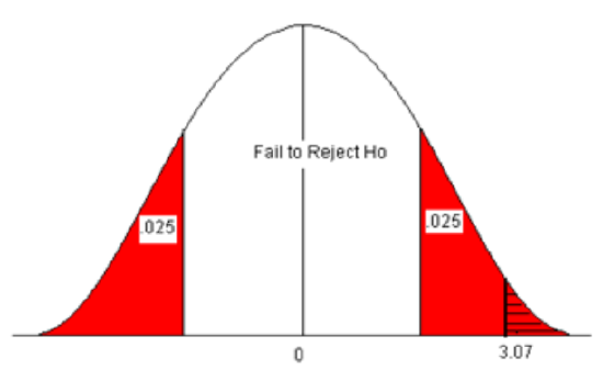
- Look up the area for the Z-score 3.07 in the standard normal table. The area (probability) is equal to 1 – 0.9989 = 0.0011.
- Multiply this by 2 to get the p-value = 2 * 0.0011 = 0.0022.
Step 4) Compare the p-value to alpha and state a conclusion.
- Use the Decision Rule (if the p-value is less than α, reject H0).
- In this problem, the p-value (0.0022) is less than alpha (0.05).
- We reject the H0. We have enough evidence to support the claim that the mean diameter growth is different from 1.35 inches/year.
Let’s look at Example 7 again.
A researcher believes that there has been an increase in the average farm size in his state since the last study five years ago. The previous study reported a mean size of 450 acres with a population standard deviation (σ) of 167 acres. He samples 45 farms and gets a sample mean of 485.8 acres. Is there enough information to support his claim?
Step 1) State the null and alternative hypotheses.
- Ho: μ = 450 acres
- H1: μ >450 acres
Step 2) State the level of significance.
- We will choose a level of significance of 5% (α = 0.05).
Step 3) Compute the test statistic.
- For this problem, the test statistic is
\[z= \frac {485.8-450}{\frac {167}{\sqrt {45}}}=1.44 \nonumber \]
The p-value is the area to the right of the Z-score 1.44 (the hatched area).
- This is equal to 1 – 0.9251 = 0.0749.
- The p-value is 0.0749.
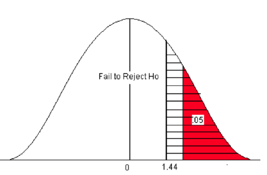
Figure \(\PageIndex{8}\): The p-value compared to the level of significance for a right-sided test.
Step 4) Compare the p-value to alpha and state a conclusion.
- Use the Decision Rule.
- In this problem, the p-value (0.0749) is greater than alpha (0.05), so we Fail to Reject the H0.
- The area of the test statistic is greater than the area of alpha (α).
We fail to reject the null hypothesis. We do not have enough evidence to support the claim that the mean farm size has increased.
Let’s look at Example 8 again.
A researcher believes that there has been a reduction in the mean number of hours that college students spend preparing for final exams. A national study stated that students at a 4-year college spend an average of 23 hours preparing for 5 final exams each semester with a population standard deviation of 7.3 hours. The researcher sampled 227 students and found a sample mean study time of 19.6 hours. Does this indicate that the average study time for final exams has decreased? Use a 1% level of significance to test this claim.
Step 1) State the null and alternative hypotheses.
- H0: μ = 23 hours
- H1: μ < 23 hours
Step 2) State the level of significance.
- This is a left-sided test so alpha (0.01) is all in the left tail.
Step 3) Compute the test statistic.
- For this problem, the test statistic is
\[z=\frac {19.6-23}{\frac {7.3}{\sqrt {227}}}=-7.02 \nonumber \]
The p-value is the area to the left of the test statistic (the little black area to the left of -7.02). The Z-score of -7.02 is not on the standard normal table. The smallest probability on the table is 0.0002. We know that the area for the Z-score -7.02 is smaller than this area (probability). Therefore, the p-value is <0.0002.
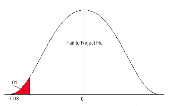
Step 4) Compare the p-value to alpha and state a conclusion.
- Use the Decision Rule.
- In this problem, the p-value (p<0.0002) is less than alpha (0.01), so we Reject the H0.
- The area of the test statistic is much less than the area of alpha (α).
We reject the null hypothesis. We have enough evidence to support the claim that the mean final exam study time has decreased below 23 hours.
Both the classical method and p-value method for testing a hypothesis will arrive at the same conclusion. In the classical method, the critical Z-score is the number on the z-axis that defines the level of significance (α). The test statistic converts the sample mean to units of standard deviation (a Z-score). If the test statistic falls in the rejection zone defined by the critical value, we will reject the null hypothesis. In this approach, two Z-scores, which are numbers on the z-axis, are compared. In the p-value approach, the p-value is the area associated with the test statistic. In this method, we compare α (which is also area under the curve) to the p-value. If the p-value is less than α, we reject the null hypothesis. The p-value is the probability of observing such a sample mean when the null hypothesis is true. If the probability is too small (less than the level of significance), then we believe we have enough statistical evidence to reject the null hypothesis and support the alternative claim.
Software Solutions
Minitab
(referring to Ex. 8)


One-Sample Z
| Test of mu = 23 vs. < 23 |
| The assumed standard deviation = 7.3 |
| 99% Upper | |||||
| N | Mean | SE Mean | Bound | Z | P |
| 227 | 19.600 | 0.485 | 20.727 | -7.02 | 0.000 |
Excel
Excel does not offer 1-sample hypothesis testing.


