3.1: The Fundamentals of Hypothesis Testing
- Page ID
- 2883
\( \newcommand{\vecs}[1]{\overset { \scriptstyle \rightharpoonup} {\mathbf{#1}} } \)
\( \newcommand{\vecd}[1]{\overset{-\!-\!\rightharpoonup}{\vphantom{a}\smash {#1}}} \)
\( \newcommand{\dsum}{\displaystyle\sum\limits} \)
\( \newcommand{\dint}{\displaystyle\int\limits} \)
\( \newcommand{\dlim}{\displaystyle\lim\limits} \)
\( \newcommand{\id}{\mathrm{id}}\) \( \newcommand{\Span}{\mathrm{span}}\)
( \newcommand{\kernel}{\mathrm{null}\,}\) \( \newcommand{\range}{\mathrm{range}\,}\)
\( \newcommand{\RealPart}{\mathrm{Re}}\) \( \newcommand{\ImaginaryPart}{\mathrm{Im}}\)
\( \newcommand{\Argument}{\mathrm{Arg}}\) \( \newcommand{\norm}[1]{\| #1 \|}\)
\( \newcommand{\inner}[2]{\langle #1, #2 \rangle}\)
\( \newcommand{\Span}{\mathrm{span}}\)
\( \newcommand{\id}{\mathrm{id}}\)
\( \newcommand{\Span}{\mathrm{span}}\)
\( \newcommand{\kernel}{\mathrm{null}\,}\)
\( \newcommand{\range}{\mathrm{range}\,}\)
\( \newcommand{\RealPart}{\mathrm{Re}}\)
\( \newcommand{\ImaginaryPart}{\mathrm{Im}}\)
\( \newcommand{\Argument}{\mathrm{Arg}}\)
\( \newcommand{\norm}[1]{\| #1 \|}\)
\( \newcommand{\inner}[2]{\langle #1, #2 \rangle}\)
\( \newcommand{\Span}{\mathrm{span}}\) \( \newcommand{\AA}{\unicode[.8,0]{x212B}}\)
\( \newcommand{\vectorA}[1]{\vec{#1}} % arrow\)
\( \newcommand{\vectorAt}[1]{\vec{\text{#1}}} % arrow\)
\( \newcommand{\vectorB}[1]{\overset { \scriptstyle \rightharpoonup} {\mathbf{#1}} } \)
\( \newcommand{\vectorC}[1]{\textbf{#1}} \)
\( \newcommand{\vectorD}[1]{\overrightarrow{#1}} \)
\( \newcommand{\vectorDt}[1]{\overrightarrow{\text{#1}}} \)
\( \newcommand{\vectE}[1]{\overset{-\!-\!\rightharpoonup}{\vphantom{a}\smash{\mathbf {#1}}}} \)
\( \newcommand{\vecs}[1]{\overset { \scriptstyle \rightharpoonup} {\mathbf{#1}} } \)
\(\newcommand{\longvect}{\overrightarrow}\)
\( \newcommand{\vecd}[1]{\overset{-\!-\!\rightharpoonup}{\vphantom{a}\smash {#1}}} \)
\(\newcommand{\avec}{\mathbf a}\) \(\newcommand{\bvec}{\mathbf b}\) \(\newcommand{\cvec}{\mathbf c}\) \(\newcommand{\dvec}{\mathbf d}\) \(\newcommand{\dtil}{\widetilde{\mathbf d}}\) \(\newcommand{\evec}{\mathbf e}\) \(\newcommand{\fvec}{\mathbf f}\) \(\newcommand{\nvec}{\mathbf n}\) \(\newcommand{\pvec}{\mathbf p}\) \(\newcommand{\qvec}{\mathbf q}\) \(\newcommand{\svec}{\mathbf s}\) \(\newcommand{\tvec}{\mathbf t}\) \(\newcommand{\uvec}{\mathbf u}\) \(\newcommand{\vvec}{\mathbf v}\) \(\newcommand{\wvec}{\mathbf w}\) \(\newcommand{\xvec}{\mathbf x}\) \(\newcommand{\yvec}{\mathbf y}\) \(\newcommand{\zvec}{\mathbf z}\) \(\newcommand{\rvec}{\mathbf r}\) \(\newcommand{\mvec}{\mathbf m}\) \(\newcommand{\zerovec}{\mathbf 0}\) \(\newcommand{\onevec}{\mathbf 1}\) \(\newcommand{\real}{\mathbb R}\) \(\newcommand{\twovec}[2]{\left[\begin{array}{r}#1 \\ #2 \end{array}\right]}\) \(\newcommand{\ctwovec}[2]{\left[\begin{array}{c}#1 \\ #2 \end{array}\right]}\) \(\newcommand{\threevec}[3]{\left[\begin{array}{r}#1 \\ #2 \\ #3 \end{array}\right]}\) \(\newcommand{\cthreevec}[3]{\left[\begin{array}{c}#1 \\ #2 \\ #3 \end{array}\right]}\) \(\newcommand{\fourvec}[4]{\left[\begin{array}{r}#1 \\ #2 \\ #3 \\ #4 \end{array}\right]}\) \(\newcommand{\cfourvec}[4]{\left[\begin{array}{c}#1 \\ #2 \\ #3 \\ #4 \end{array}\right]}\) \(\newcommand{\fivevec}[5]{\left[\begin{array}{r}#1 \\ #2 \\ #3 \\ #4 \\ #5 \\ \end{array}\right]}\) \(\newcommand{\cfivevec}[5]{\left[\begin{array}{c}#1 \\ #2 \\ #3 \\ #4 \\ #5 \\ \end{array}\right]}\) \(\newcommand{\mattwo}[4]{\left[\begin{array}{rr}#1 \amp #2 \\ #3 \amp #4 \\ \end{array}\right]}\) \(\newcommand{\laspan}[1]{\text{Span}\{#1\}}\) \(\newcommand{\bcal}{\cal B}\) \(\newcommand{\ccal}{\cal C}\) \(\newcommand{\scal}{\cal S}\) \(\newcommand{\wcal}{\cal W}\) \(\newcommand{\ecal}{\cal E}\) \(\newcommand{\coords}[2]{\left\{#1\right\}_{#2}}\) \(\newcommand{\gray}[1]{\color{gray}{#1}}\) \(\newcommand{\lgray}[1]{\color{lightgray}{#1}}\) \(\newcommand{\rank}{\operatorname{rank}}\) \(\newcommand{\row}{\text{Row}}\) \(\newcommand{\col}{\text{Col}}\) \(\renewcommand{\row}{\text{Row}}\) \(\newcommand{\nul}{\text{Nul}}\) \(\newcommand{\var}{\text{Var}}\) \(\newcommand{\corr}{\text{corr}}\) \(\newcommand{\len}[1]{\left|#1\right|}\) \(\newcommand{\bbar}{\overline{\bvec}}\) \(\newcommand{\bhat}{\widehat{\bvec}}\) \(\newcommand{\bperp}{\bvec^\perp}\) \(\newcommand{\xhat}{\widehat{\xvec}}\) \(\newcommand{\vhat}{\widehat{\vvec}}\) \(\newcommand{\uhat}{\widehat{\uvec}}\) \(\newcommand{\what}{\widehat{\wvec}}\) \(\newcommand{\Sighat}{\widehat{\Sigma}}\) \(\newcommand{\lt}{<}\) \(\newcommand{\gt}{>}\) \(\newcommand{\amp}{&}\) \(\definecolor{fillinmathshade}{gray}{0.9}\)The previous two chapters introduced methods for organizing and summarizing sample data, and using sample statistics to estimate population parameters. This chapter introduces the next major topic of inferential statistics: hypothesis testing.
A hypothesis is a statement or claim about a property of a population.
The Fundamentals of Hypothesis Testing
When conducting scientific research, typically there is some known information, perhaps from some past work or from a long accepted idea. We want to test whether this claim is believable. This is the basic idea behind a hypothesis test:
- State what we think is true.
- Quantify how confident we are about our claim.
- Use sample statistics to make inferences about population parameters.
For example, past research tells us that the average life span for a hummingbird is about four years. You have been studying the hummingbirds in the southeastern United States and find a sample mean lifespan of 4.8 years. Should you reject the known or accepted information in favor of your results? How confident are you in your estimate? At what point would you say that there is enough evidence to reject the known information and support your alternative claim? How far from the known mean of four years can the sample mean be before we reject the idea that the average lifespan of a hummingbird is four years?
Hypothesis testing is a procedure, based on sample evidence and probability, used to test claims regarding a characteristic of a population.
A hypothesis is a claim or statement about a characteristic of a population of interest to us. A hypothesis test is a way for us to use our sample statistics to test a specific claim.
The population mean weight is known to be 157 lb. We want to test the claim that the mean weight has increased.
Two years ago, the proportion of infected plants was 37%. We believe that a treatment has helped, and we want to test the claim that there has been a reduction in the proportion of infected plants.
Components of a Formal Hypothesis Test
The null hypothesis is a statement about the value of a population parameter, such as the population mean (µ) or the population proportion (p). It contains the condition of equality and is denoted as H0 (H-naught).
H0 : µ = 157 or H0 : p = 0.37
The alternative hypothesis is the claim to be tested, the opposite of the null hypothesis. It contains the value of the parameter that we consider plausible and is denoted as H1 .
H1 : µ > 157 or H1 : p ≠ 0.37
The test statistic is a value computed from the sample data that is used in making a decision about the rejection of the null hypothesis. The test statistic converts the sample mean (x̄) or sample proportion (p̂) to a Z- or t-score under the assumption that the null hypothesis is true. It is used to decide whether the difference between the sample statistic and the hypothesized claim is significant.
The p-value is the area under the curve to the left or right of the test statistic. It is compared to the level of significance (α).
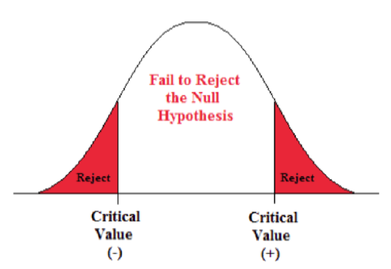
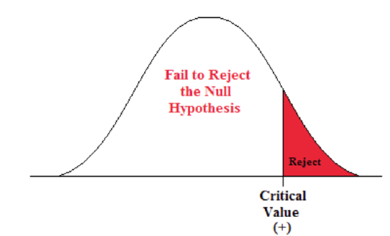
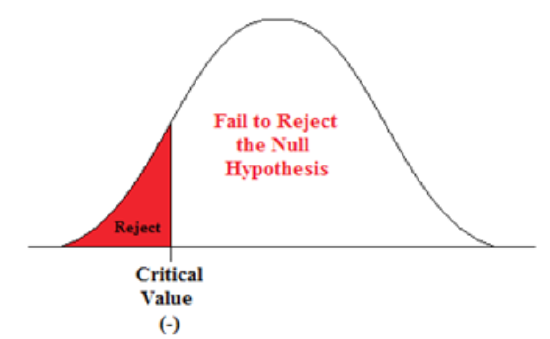
The critical value is the value that defines the rejection zone (the test statistic values that would lead to rejection of the null hypothesis). It is defined by the level of significance.
The level of significance (α) is the probability that the test statistic will fall into the critical region when the null hypothesis is true. This level is set by the researcher.
The conclusion is the final decision of the hypothesis test. The conclusion must always be clearly stated, communicating the decision based on the components of the test. It is important to realize that we never prove or accept the null hypothesis. We are merely saying that the sample evidence is not strong enough to warrant the rejection of the null hypothesis. The conclusion is made up of two parts:
1) Reject or fail to reject the null hypothesis, and 2) there is or is not enough evidence to support the alternative claim.
Option 1) Reject the null hypothesis (H0). This means that you have enough statistical evidence to support the alternative claim (H1).
Option 2) Fail to reject the null hypothesis (H0). This means that you do NOT have enough evidence to support the alternative claim (H1).
Another way to think about hypothesis testing is to compare it to the US justice system. A defendant is innocent until proven guilty (Null hypothesis—innocent). The prosecuting attorney tries to prove that the defendant is guilty (Alternative hypothesis—guilty). There are two possible conclusions that the jury can reach. First, the defendant is guilty (Reject the null hypothesis). Second, the defendant is not guilty (Fail to reject the null hypothesis). This is NOT the same thing as saying the defendant is innocent! In the first case, the prosecutor had enough evidence to reject the null hypothesis (innocent) and support the alternative claim (guilty). In the second case, the prosecutor did NOT have enough evidence to reject the null hypothesis (innocent) and support the alternative claim of guilty.
The Null and Alternative Hypotheses
There are three different pairs of null and alternative hypotheses:
Table \(PageIndex{1}\): The rejection zone for a two-sided hypothesis test.
|
Two-sided |
Left-sided |
Right-sided |
|---|---|---|
|
\(\mathrm{H}_{\mathrm{O}}: \boldsymbol{\mu}=\mathrm{c}\) |
\(\mathbf{H}_{\mathbf{0}}: \boldsymbol{\mu}=\mathbf{C}\) |
\(\mathbf{H}_{\mathbf{0}}: \boldsymbol{\mu}=\mathbf{C}\) |
|
\(\mathbf{H}_{\mathbf{1}}: \boldsymbol{\mu \neq \mathbf { C }}\) |
\(\mathbf{H}_{\mathbf{1}}: \boldsymbol{\mu}< \mathbf{C}\) |
\(\mathbf{H}_{\mathbf{1}}: \boldsymbol{\mu}>\mathbf{C}\) |
where c is some known value.
A Two-sided Test
This tests whether the population parameter is equal to, versus not equal to, some specific value.
Ho: μ = 12 vs. H1: μ ≠ 12
The critical region is divided equally into the two tails and the critical values are ± values that define the rejection zones.

A forester studying diameter growth of red pine believes that the mean diameter growth will be different if a fertilization treatment is applied to the stand.
- Ho: μ = 1.2 in./ year
- H1: μ ≠ 1.2 in./ year
This is a two-sided question, as the forester doesn’t state whether population mean diameter growth will increase or decrease.
A Right-sided Test
This tests whether the population parameter is equal to, versus greater than, some specific value.
Ho: μ = 12 vs. H1: μ > 12
The critical region is in the right tail and the critical value is a positive value that defines the rejection zone.

A biologist believes that there has been an increase in the mean number of lakes infected with milfoil, an invasive species, since the last study five years ago.
- Ho: μ = 15 lakes
- H1: μ >15 lakes
This is a right-sided question, as the biologist believes that there has been an increase in population mean number of infected lakes.
A Left-sided Test
This tests whether the population parameter is equal to, versus less than, some specific value.
Ho: μ = 12 vs. H1: μ < 12
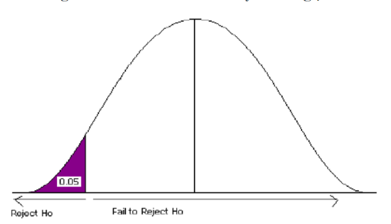
The critical region is in the left tail and the critical value is a negative value that defines the rejection zone.

A scientist’s research indicates that there has been a change in the proportion of people who support certain environmental policies. He wants to test the claim that there has been a reduction in the proportion of people who support these policies.
- Ho: p = 0.57
- H1: p < 0.57
This is a left-sided question, as the scientist believes that there has been a reduction in the true population proportion.
Statistically Significant
When the observed results (the sample statistics) are unlikely (a low probability) under the assumption that the null hypothesis is true, we say that the result is statistically significant, and we reject the null hypothesis. This result depends on the level of significance, the sample statistic, sample size, and whether it is a one- or two-sided alternative hypothesis.
Types of Errors
When testing, we arrive at a conclusion of rejecting the null hypothesis or failing to reject the null hypothesis. Such conclusions are sometimes correct and sometimes incorrect (even when we have followed all the correct procedures). We use incomplete sample data to reach a conclusion and there is always the possibility of reaching the wrong conclusion. There are four possible conclusions to reach from hypothesis testing. Of the four possible outcomes, two are correct and two are NOT correct.
Table \(\PageIndex{2}\). Possible outcomes from a hypothesis test.
|
H0 is True |
H1 is True |
|
|---|---|---|
|
Do Not Reject H0 |
Correct Conclusion |
Type II Error |
|
Reject H0 |
Type I Error |
Correct Conclusion |
A Type I error is when we reject the null hypothesis when it is true. The symbol α (alpha) is used to represent Type I errors. This is the same alpha we use as the level of significance. By setting alpha as low as reasonably possible, we try to control the Type I error through the level of significance.
A Type II error is when we fail to reject the null hypothesis when it is false. The symbol β(beta) is used to represent Type II errors.
In general, Type I errors are considered more serious. One step in the hypothesis test procedure involves selecting the significance level (α), which is the probability of rejecting the null hypothesis when it is correct. So the researcher can select the level of significance that minimizes Type I errors. However, there is a mathematical relationship between α, β, and n (sample size).
- As α increases, β decreases
- As α decreases, β increases
- As sample size increases (n), both α and β decrease
The natural inclination is to select the smallest possible value for α, thinking to minimize the possibility of causing a Type I error. Unfortunately, this forces an increase in Type II errors. By making the rejection zone too small, you may fail to reject the null hypothesis, when, in fact, it is false. Typically, we select the best sample size and level of significance, automatically setting β.

Figure 4.
Power of the Test
A Type II error (β) is the probability of failing to reject a false null hypothesis. It follows that 1-β is the probability of rejecting a false null hypothesis. This probability is identified as the power of the test, and is often used to gauge the test’s effectiveness in recognizing that a null hypothesis is false.
The probability that at a fixed level α significance test will reject H0, when a particular alternative value of the parameter is true is called the power of the test.
Power is also directly linked to sample size. For example, suppose the null hypothesis is that the mean fish weight is 8.7 lb. Given sample data, a level of significance of 5%, and an alternative weight of 9.2 lb., we can compute the power of the test to reject μ = 8.7 lb. If we have a small sample size, the power will be low. However, increasing the sample size will increase the power of the test. Increasing the level of significance will also increase power. A 5% test of significance will have a greater chance of rejecting the null hypothesis than a 1% test because the strength of evidence required for the rejection is less. Decreasing the standard deviation has the same effect as increasing the sample size: there is more information about μ.


