3.4: Hypothesis Test for a Population Proportion
- Page ID
- 2886
\( \newcommand{\vecs}[1]{\overset { \scriptstyle \rightharpoonup} {\mathbf{#1}} } \)
\( \newcommand{\vecd}[1]{\overset{-\!-\!\rightharpoonup}{\vphantom{a}\smash {#1}}} \)
\( \newcommand{\id}{\mathrm{id}}\) \( \newcommand{\Span}{\mathrm{span}}\)
( \newcommand{\kernel}{\mathrm{null}\,}\) \( \newcommand{\range}{\mathrm{range}\,}\)
\( \newcommand{\RealPart}{\mathrm{Re}}\) \( \newcommand{\ImaginaryPart}{\mathrm{Im}}\)
\( \newcommand{\Argument}{\mathrm{Arg}}\) \( \newcommand{\norm}[1]{\| #1 \|}\)
\( \newcommand{\inner}[2]{\langle #1, #2 \rangle}\)
\( \newcommand{\Span}{\mathrm{span}}\)
\( \newcommand{\id}{\mathrm{id}}\)
\( \newcommand{\Span}{\mathrm{span}}\)
\( \newcommand{\kernel}{\mathrm{null}\,}\)
\( \newcommand{\range}{\mathrm{range}\,}\)
\( \newcommand{\RealPart}{\mathrm{Re}}\)
\( \newcommand{\ImaginaryPart}{\mathrm{Im}}\)
\( \newcommand{\Argument}{\mathrm{Arg}}\)
\( \newcommand{\norm}[1]{\| #1 \|}\)
\( \newcommand{\inner}[2]{\langle #1, #2 \rangle}\)
\( \newcommand{\Span}{\mathrm{span}}\) \( \newcommand{\AA}{\unicode[.8,0]{x212B}}\)
\( \newcommand{\vectorA}[1]{\vec{#1}} % arrow\)
\( \newcommand{\vectorAt}[1]{\vec{\text{#1}}} % arrow\)
\( \newcommand{\vectorB}[1]{\overset { \scriptstyle \rightharpoonup} {\mathbf{#1}} } \)
\( \newcommand{\vectorC}[1]{\textbf{#1}} \)
\( \newcommand{\vectorD}[1]{\overrightarrow{#1}} \)
\( \newcommand{\vectorDt}[1]{\overrightarrow{\text{#1}}} \)
\( \newcommand{\vectE}[1]{\overset{-\!-\!\rightharpoonup}{\vphantom{a}\smash{\mathbf {#1}}}} \)
\( \newcommand{\vecs}[1]{\overset { \scriptstyle \rightharpoonup} {\mathbf{#1}} } \)
\( \newcommand{\vecd}[1]{\overset{-\!-\!\rightharpoonup}{\vphantom{a}\smash {#1}}} \)
\(\newcommand{\avec}{\mathbf a}\) \(\newcommand{\bvec}{\mathbf b}\) \(\newcommand{\cvec}{\mathbf c}\) \(\newcommand{\dvec}{\mathbf d}\) \(\newcommand{\dtil}{\widetilde{\mathbf d}}\) \(\newcommand{\evec}{\mathbf e}\) \(\newcommand{\fvec}{\mathbf f}\) \(\newcommand{\nvec}{\mathbf n}\) \(\newcommand{\pvec}{\mathbf p}\) \(\newcommand{\qvec}{\mathbf q}\) \(\newcommand{\svec}{\mathbf s}\) \(\newcommand{\tvec}{\mathbf t}\) \(\newcommand{\uvec}{\mathbf u}\) \(\newcommand{\vvec}{\mathbf v}\) \(\newcommand{\wvec}{\mathbf w}\) \(\newcommand{\xvec}{\mathbf x}\) \(\newcommand{\yvec}{\mathbf y}\) \(\newcommand{\zvec}{\mathbf z}\) \(\newcommand{\rvec}{\mathbf r}\) \(\newcommand{\mvec}{\mathbf m}\) \(\newcommand{\zerovec}{\mathbf 0}\) \(\newcommand{\onevec}{\mathbf 1}\) \(\newcommand{\real}{\mathbb R}\) \(\newcommand{\twovec}[2]{\left[\begin{array}{r}#1 \\ #2 \end{array}\right]}\) \(\newcommand{\ctwovec}[2]{\left[\begin{array}{c}#1 \\ #2 \end{array}\right]}\) \(\newcommand{\threevec}[3]{\left[\begin{array}{r}#1 \\ #2 \\ #3 \end{array}\right]}\) \(\newcommand{\cthreevec}[3]{\left[\begin{array}{c}#1 \\ #2 \\ #3 \end{array}\right]}\) \(\newcommand{\fourvec}[4]{\left[\begin{array}{r}#1 \\ #2 \\ #3 \\ #4 \end{array}\right]}\) \(\newcommand{\cfourvec}[4]{\left[\begin{array}{c}#1 \\ #2 \\ #3 \\ #4 \end{array}\right]}\) \(\newcommand{\fivevec}[5]{\left[\begin{array}{r}#1 \\ #2 \\ #3 \\ #4 \\ #5 \\ \end{array}\right]}\) \(\newcommand{\cfivevec}[5]{\left[\begin{array}{c}#1 \\ #2 \\ #3 \\ #4 \\ #5 \\ \end{array}\right]}\) \(\newcommand{\mattwo}[4]{\left[\begin{array}{rr}#1 \amp #2 \\ #3 \amp #4 \\ \end{array}\right]}\) \(\newcommand{\laspan}[1]{\text{Span}\{#1\}}\) \(\newcommand{\bcal}{\cal B}\) \(\newcommand{\ccal}{\cal C}\) \(\newcommand{\scal}{\cal S}\) \(\newcommand{\wcal}{\cal W}\) \(\newcommand{\ecal}{\cal E}\) \(\newcommand{\coords}[2]{\left\{#1\right\}_{#2}}\) \(\newcommand{\gray}[1]{\color{gray}{#1}}\) \(\newcommand{\lgray}[1]{\color{lightgray}{#1}}\) \(\newcommand{\rank}{\operatorname{rank}}\) \(\newcommand{\row}{\text{Row}}\) \(\newcommand{\col}{\text{Col}}\) \(\renewcommand{\row}{\text{Row}}\) \(\newcommand{\nul}{\text{Nul}}\) \(\newcommand{\var}{\text{Var}}\) \(\newcommand{\corr}{\text{corr}}\) \(\newcommand{\len}[1]{\left|#1\right|}\) \(\newcommand{\bbar}{\overline{\bvec}}\) \(\newcommand{\bhat}{\widehat{\bvec}}\) \(\newcommand{\bperp}{\bvec^\perp}\) \(\newcommand{\xhat}{\widehat{\xvec}}\) \(\newcommand{\vhat}{\widehat{\vvec}}\) \(\newcommand{\uhat}{\widehat{\uvec}}\) \(\newcommand{\what}{\widehat{\wvec}}\) \(\newcommand{\Sighat}{\widehat{\Sigma}}\) \(\newcommand{\lt}{<}\) \(\newcommand{\gt}{>}\) \(\newcommand{\amp}{&}\) \(\definecolor{fillinmathshade}{gray}{0.9}\)Hypothesis Test for a Population Proportion (p)
Frequently, the parameter we are testing is the population proportion.
- We are studying the proportion of trees with cavities for wildlife habitat.
- We need to know if the proportion of people who support green building materials has changed.
- Has the proportion of wolves that died last year in Yellowstone increased from the year before?
Recall that the best point estimate of p, the population proportion, is given by
\[\hat {p} = \dfrac {x}{n}\]
where x is the number of individuals in the sample with the characteristic studied and n is the sample size. The sampling distribution of p̂ is approximately normal with a mean \(\mu_{\hat {p}} = p\) and a standard deviation
\[\sigma_{\hat {p}} = \sqrt {\dfrac {p(1-p)}{n}}\]
when np(1 – p)≥10. We can use both the classical approach and the p-value approach for testing.
The steps for a hypothesis test are the same that we covered in Section 2.
- State the null and alternative hypotheses.
- State the level of significance and the critical value.
- Compute the test statistic.
- State a conclusion.
The test statistic follows the standard normal distribution. Notice that the standard error (the denominator) uses p instead of p̂, which was used when constructing a confidence interval about the population proportion. In a hypothesis test, the null hypothesis is assumed to be true, so the known proportion is used.
\[ z= \dfrac {\hat {p} - p} {\sqrt {\dfrac {p(1-p)}{n}}}\]
- The critical value comes from the standard normal table, just as in Section 2. We will still use the same three pairs of null and alternative hypotheses as we used in the previous sections, but the parameter is now p instead of μ:
Table \(PageIndex{1}\): The rejection zone for a two-sided hypothesis test.
|
Two-sided |
Left-sided |
Right-sided |
|---|---|---|
|
\(\mathrm{H}_{\mathrm{O}}: \boldsymbol{p}=\mathrm{c}\) |
\(\mathbf{H}_{\mathbf{0}}: \boldsymbol{p}=\mathbf{C}\) |
\(\mathbf{H}_{\mathbf{0}}: \boldsymbol{p}=\mathbf{C}\) |
|
\(\mathbf{H}_{\mathbf{1}}: \boldsymbol{p \neq \mathbf { C }}\) |
\(\mathbf{H}_{\mathbf{1}}: \boldsymbol{p}< \mathbf{C}\) |
\(\mathbf{H}_{\mathbf{1}}: \boldsymbol{p}>\mathbf{C}\) |
- For a two-sided test, alpha will be divided by 2 giving a ± Zα/2 critical value.
- For a left-sided test, alpha will be all in the left tail giving a – Zα critical value.
- For a right-sided test, alpha will be all in the right tail giving a Zα critical value.
botanist has produced a new variety of hybrid soy plant that is better able to withstand drought than other varieties. The botanist knows the seed germination for the parent plants is 75%, but does not know the seed germination for the new hybrid. He tests the claim that it is different from the parent plants. To test this claim, 450 seeds from the hybrid plant are tested and 321 have germinated. Use a 5% level of significance to test this claim that the germination rate is different from 75%.
Solution
Step 1) State the null and alternative hypotheses.
- Ho: p = 0.75
- H1: p ≠ 0.75
Step 2) State the level of significance and the critical value.
This is a two-sided question so alpha is divided by 2.
- Alpha is 0.05 so the critical values are ± Zα/2 = ± Z.025.
- Look on the negative side of the standard normal table, in the body of values for 0.025.
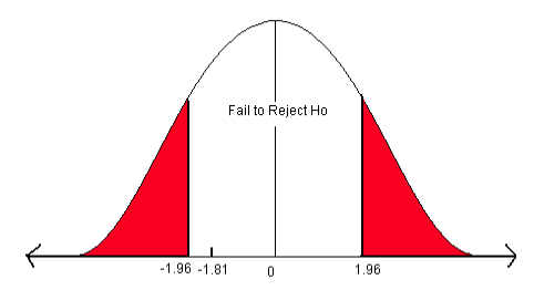
- The critical values are ± 1.96.
Step 3) Compute the test statistic.
- The test statistic is the number of standard deviations the sample mean is from the known mean. It is also a Z-score, just like the critical value.
\[ z= \dfrac {\hat {p} - p} {\sqrt {\dfrac {p(1-p)}{n}}}\]
- For this problem, the test statistic is
\[z=\dfrac {0.713-0.75}{\sqrt {\dfrac {0.75(1-0.75)}{450}}} = -1.81 \nonumber \]
Step 4) State a conclusion.
- Compare the test statistic to the critical value.

The test statistic does not fall in the rejection zone. We fail to reject the null hypothesis. We do not have enough evidence to support the claim that the germination rate of the hybrid plant is different from the parent plants.
Let’s answer this question using the p-value approach. Remember, for a two-sided alternative hypothesis (“not equal”), the p-value is two times the area of the test statistic. The test statistic is -1.81 and we want to find the area to the left of -1.81 from the standard normal table.
- On the negative page, find the Z-score -1.81. Find the area associated with this Z-score.
- The area = 0.0351.
- This is a two-sided test so multiply the area times 2 to get the p-value = 0.0351 x 2 = 0.0702.
Now compare the p-value to alpha. The Decision Rule states that if the p-value is less than alpha, reject the H0. In this case, the p-value (0.0702) is greater than alpha (0.05) so we will fail to reject H0. We do not have enough evidence to support the claim that the germination rate of the hybrid plant is different from the parent plants.
You are a biologist studying the wildlife habitat in the Monongahela National Forest. Cavities in older trees provide excellent habitat for a variety of birds and small mammals. A study five years ago stated that 32% of the trees in this forest had suitable cavities for this type of wildlife. You believe that the proportion of cavity trees has increased. You sample 196 trees and find that 79 trees have cavities. Does this evidence support your claim that there has been an increase in the proportion of cavity trees?
Use a 10% level of significance to test this claim.
Solution
Step 1) State the null and alternative hypotheses.
- Ho: p = 0.32
- H1: p > 0.32
Step 2) State the level of significance and the critical value.
This is a one-sided question so alpha is divided by 1.
- Alpha is 0.10 so the critical value is Zα = Z .10
- Look on the positive side of the standard normal table, in the body of values for 0.90.
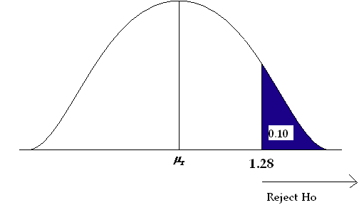
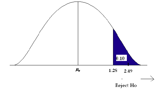
- The critical value is 1.28.

Step 3) Compute the test statistic.
- The test statistic is the number of standard deviations the sample proportion is from the known proportion. It is also a Z-score, just like the critical value.
\[ z= \dfrac {\hat {p} - p} {\sqrt {\dfrac {p(1-p)}{n}}}\]
- For this problem, the test statistic is:
\[z= \frac {0.403-0.32}{\sqrt {\frac {0.32(1-0.32)}{196}}}=2.49 \nonumber \]
Step 4) State a conclusion.
- Compare the test statistic to the critical value.

The test statistic is larger than the critical value (it falls in the rejection zone). We will reject the null hypothesis. We have enough evidence to support the claim that there has been an increase in the proportion of cavity trees.
Now use the p-value approach to answer the question. This is a right-sided question (“greater than”), so the p-value is equal to the area to the right of the test statistic. Go to the positive side of the standard normal table and find the area associated with the Z-score of 2.49. The area is 0.9936. Remember that this table is cumulative from the left. To find the area to the right of 2.49, we subtract from one.
p-value = (1 – 0.9936) = 0.0064
The p-value is less than the level of significance (0.10), so we reject the null hypothesis. We have enough evidence to support the claim that the proportion of cavity trees has increased.
Software Solutions
Minitab
(referring to Ex. 15)


Test and CI for One Proportion
Test of p = 0.32 vs. p > 0.32
90% Lower
| Sample | X | N | Sample p | Bound | Z-Value | p-Value |
|---|---|---|---|---|---|---|
| 1 | 79 | 196 | 0.403061 | 0.358160 | 2.49 | 0.006 |
| Using the normal approximation. | ||||||
Excel
Excel does not offer 1-sample hypothesis testing.


