
15.3: Wilcoxon signed-rank test
- Page ID
- 45238

\( \newcommand{\vecs}[1]{\overset { \scriptstyle \rightharpoonup} {\mathbf{#1}} } \)
\( \newcommand{\vecd}[1]{\overset{-\!-\!\rightharpoonup}{\vphantom{a}\smash {#1}}} \)
\( \newcommand{\dsum}{\displaystyle\sum\limits} \)
\( \newcommand{\dint}{\displaystyle\int\limits} \)
\( \newcommand{\dlim}{\displaystyle\lim\limits} \)
\( \newcommand{\id}{\mathrm{id}}\) \( \newcommand{\Span}{\mathrm{span}}\)
( \newcommand{\kernel}{\mathrm{null}\,}\) \( \newcommand{\range}{\mathrm{range}\,}\)
\( \newcommand{\RealPart}{\mathrm{Re}}\) \( \newcommand{\ImaginaryPart}{\mathrm{Im}}\)
\( \newcommand{\Argument}{\mathrm{Arg}}\) \( \newcommand{\norm}[1]{\| #1 \|}\)
\( \newcommand{\inner}[2]{\langle #1, #2 \rangle}\)
\( \newcommand{\Span}{\mathrm{span}}\)
\( \newcommand{\id}{\mathrm{id}}\)
\( \newcommand{\Span}{\mathrm{span}}\)
\( \newcommand{\kernel}{\mathrm{null}\,}\)
\( \newcommand{\range}{\mathrm{range}\,}\)
\( \newcommand{\RealPart}{\mathrm{Re}}\)
\( \newcommand{\ImaginaryPart}{\mathrm{Im}}\)
\( \newcommand{\Argument}{\mathrm{Arg}}\)
\( \newcommand{\norm}[1]{\| #1 \|}\)
\( \newcommand{\inner}[2]{\langle #1, #2 \rangle}\)
\( \newcommand{\Span}{\mathrm{span}}\) \( \newcommand{\AA}{\unicode[.8,0]{x212B}}\)
\( \newcommand{\vectorA}[1]{\vec{#1}} % arrow\)
\( \newcommand{\vectorAt}[1]{\vec{\text{#1}}} % arrow\)
\( \newcommand{\vectorB}[1]{\overset { \scriptstyle \rightharpoonup} {\mathbf{#1}} } \)
\( \newcommand{\vectorC}[1]{\textbf{#1}} \)
\( \newcommand{\vectorD}[1]{\overrightarrow{#1}} \)
\( \newcommand{\vectorDt}[1]{\overrightarrow{\text{#1}}} \)
\( \newcommand{\vectE}[1]{\overset{-\!-\!\rightharpoonup}{\vphantom{a}\smash{\mathbf {#1}}}} \)
\( \newcommand{\vecs}[1]{\overset { \scriptstyle \rightharpoonup} {\mathbf{#1}} } \)
\(\newcommand{\longvect}{\overrightarrow}\)
\( \newcommand{\vecd}[1]{\overset{-\!-\!\rightharpoonup}{\vphantom{a}\smash {#1}}} \)
\(\newcommand{\avec}{\mathbf a}\) \(\newcommand{\bvec}{\mathbf b}\) \(\newcommand{\cvec}{\mathbf c}\) \(\newcommand{\dvec}{\mathbf d}\) \(\newcommand{\dtil}{\widetilde{\mathbf d}}\) \(\newcommand{\evec}{\mathbf e}\) \(\newcommand{\fvec}{\mathbf f}\) \(\newcommand{\nvec}{\mathbf n}\) \(\newcommand{\pvec}{\mathbf p}\) \(\newcommand{\qvec}{\mathbf q}\) \(\newcommand{\svec}{\mathbf s}\) \(\newcommand{\tvec}{\mathbf t}\) \(\newcommand{\uvec}{\mathbf u}\) \(\newcommand{\vvec}{\mathbf v}\) \(\newcommand{\wvec}{\mathbf w}\) \(\newcommand{\xvec}{\mathbf x}\) \(\newcommand{\yvec}{\mathbf y}\) \(\newcommand{\zvec}{\mathbf z}\) \(\newcommand{\rvec}{\mathbf r}\) \(\newcommand{\mvec}{\mathbf m}\) \(\newcommand{\zerovec}{\mathbf 0}\) \(\newcommand{\onevec}{\mathbf 1}\) \(\newcommand{\real}{\mathbb R}\) \(\newcommand{\twovec}[2]{\left[\begin{array}{r}#1 \\ #2 \end{array}\right]}\) \(\newcommand{\ctwovec}[2]{\left[\begin{array}{c}#1 \\ #2 \end{array}\right]}\) \(\newcommand{\threevec}[3]{\left[\begin{array}{r}#1 \\ #2 \\ #3 \end{array}\right]}\) \(\newcommand{\cthreevec}[3]{\left[\begin{array}{c}#1 \\ #2 \\ #3 \end{array}\right]}\) \(\newcommand{\fourvec}[4]{\left[\begin{array}{r}#1 \\ #2 \\ #3 \\ #4 \end{array}\right]}\) \(\newcommand{\cfourvec}[4]{\left[\begin{array}{c}#1 \\ #2 \\ #3 \\ #4 \end{array}\right]}\) \(\newcommand{\fivevec}[5]{\left[\begin{array}{r}#1 \\ #2 \\ #3 \\ #4 \\ #5 \\ \end{array}\right]}\) \(\newcommand{\cfivevec}[5]{\left[\begin{array}{c}#1 \\ #2 \\ #3 \\ #4 \\ #5 \\ \end{array}\right]}\) \(\newcommand{\mattwo}[4]{\left[\begin{array}{rr}#1 \amp #2 \\ #3 \amp #4 \\ \end{array}\right]}\) \(\newcommand{\laspan}[1]{\text{Span}\{#1\}}\) \(\newcommand{\bcal}{\cal B}\) \(\newcommand{\ccal}{\cal C}\) \(\newcommand{\scal}{\cal S}\) \(\newcommand{\wcal}{\cal W}\) \(\newcommand{\ecal}{\cal E}\) \(\newcommand{\coords}[2]{\left\{#1\right\}_{#2}}\) \(\newcommand{\gray}[1]{\color{gray}{#1}}\) \(\newcommand{\lgray}[1]{\color{lightgray}{#1}}\) \(\newcommand{\rank}{\operatorname{rank}}\) \(\newcommand{\row}{\text{Row}}\) \(\newcommand{\col}{\text{Col}}\) \(\renewcommand{\row}{\text{Row}}\) \(\newcommand{\nul}{\text{Nul}}\) \(\newcommand{\var}{\text{Var}}\) \(\newcommand{\corr}{\text{corr}}\) \(\newcommand{\len}[1]{\left|#1\right|}\) \(\newcommand{\bbar}{\overline{\bvec}}\) \(\newcommand{\bhat}{\widehat{\bvec}}\) \(\newcommand{\bperp}{\bvec^\perp}\) \(\newcommand{\xhat}{\widehat{\xvec}}\) \(\newcommand{\vhat}{\widehat{\vvec}}\) \(\newcommand{\uhat}{\widehat{\uvec}}\) \(\newcommand{\what}{\widehat{\wvec}}\) \(\newcommand{\Sighat}{\widehat{\Sigma}}\) \(\newcommand{\lt}{<}\) \(\newcommand{\gt}{>}\) \(\newcommand{\amp}{&}\) \(\definecolor{fillinmathshade}{gray}{0.9}\)Introduction
When experimental units are repeated or paired, they lack independence and evaluating any difference between paired groups without accounting for the association between the repeat measures or between the pairs of related subjects would lead to incorrect inferences. A familiar pairing of experimental units occurs in clinical observational research in which control subjects and treatment subjects are matched by many characteristics.
In such cases, the parametric paired \(t\)-test would be used to evaluate inferences about the differences between repeat measures or between treatment and matched control subjects for some measured outcome. A nonparametric alternative to the paired \(t\)-test is the Wilcoxon signed rank test, also called the paired Wilcoxon test.
Another common example of paired sampling units would be that individuals are measured more than once for the same character or feature. For example, in Chapter 10.3 we presented results of running pace in minutes to complete the race of 15 women for repeated trials (in different years) at a 5K race held annually in Honolulu (Table 1).
| ID | Race 1 | Race 2 |
| 1 | 15.28 | 15.61 |
| 2 | 11.22 | 11.19 |
| 3 | 8.80 | 9.14 |
| 4 | 8.88 | 5.46 |
| 5 | 9.81 | 10.50 |
| 6 | 6.12 | 5.69 |
| 7 | 8.31 | 8.71 |
| 8 | 6.26 | 7.42 |
| 9 | 17.16 | 16.41 |
| 10 | 16.23 | 15.82 |
| 11 | 5.90 | 7.12 |
| 12 | 8.31 | 10.48 |
| 13 | 5.93 | 8.64 |
| 14 | 10.54 | 5.99 |
| 15 | 9.53 | 8.69 |
To get the paired Wilcoxon test in R Commander, select Rcmdr: Statistics → Nonparametric tests → Paired Wilcoxon Test
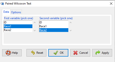
Select first variable (e.g., Race1), second variable (e.g., Race2). Next, select Options tab and set null hypothesis. Accept defaults (Fig. \(\PageIndex{2}\)).
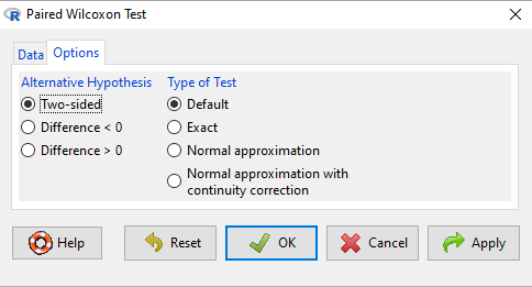
For the nonparametric paired Wilcoxon test we choose among the options to set our conditions; from the context menu a two-tailed test and we elect to use the defaults for the tests and calculations of p-values.
The results, copied from the Output window, are shown below. The calculation of the Wilcoxon test statistic (V) is straightforward, involving summing the ranks. Obtaining the p-value of the test of the null is a bit more involved as it depends on permutations of all possible combinations of differences. For us, R will do nicely with the details, and we just need to check the p-value.
with(repeat15_banana5K, wilcox.test(Race.1, Race.2, alternative='two.sided', paired=TRUE))
# median difference
[1] -0.3313126

Wilcoxon signed rank exact test
data: Race.1 and Race.2
V = 58, p-value = 0.9341
alternative hypothesis: true location shift is not equal to 0
End R output
Here, we see that the median difference is small (-0.33), and the associated p-value is 0.93. Thus, we failed to reject the null hypothesis and should conclude that there was no difference in median running pace during the first and second trials.
Note that this is the same general conclusion we got when we ran a paired \(t\)-test on this data set: no difference between day one and day two.
R code
example.ch10.3 <- read.table(header=TRUE, text = "
ID Race1 Race2
1 15.28 15.61
2 11.22 11.19
3 8.80 9.14
4 8.88 5.46
5 9.81 10.50
6 6.12 5.69
7 8.31 8.71
8 6.26 7.42
9 17.16 16.41
10 16.23 15.82
11 5.90 7.12
12 8.31 10.48
13 5.93 8.64
14 10.54 5.99
15 9.53 8.69
")
Questions
- This question lists all fourteen statistical tests we have been introduced to so far
a. Mark yes or no as to whether or not the test is a parametric test
b. Identify the nonparametric test(s) with their equivalent parametric test(s). If there are no equivalency, simply write “none.”Parametric test?
Yes/NoIf nonparametric, write the number(s) of the tests that the nonparametric test serves as an alternate for 1. ANOVA by ranks 2. Bartlett Test 3. Chi-squared contingency table 4. Chi-squared goodness of fit 5. Fisher Exact test 6. Independent-sample \(t\)-test 7. Kruskal-Walis test 8. Levene test 9. One-sample \(t\)-test 10. One-way ANOVA 11. Paired \(t\)-test 12. Shapiro-Wilks test 13. Tukey post-hoc comparisons 14. Welch’s test