15.2: Wilcoxon rank sum test

Introduction

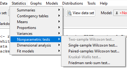
Wilcoxon rank sum test, also called the two-sample Wilcoxon test, is a nonparametric test. It is equivalent to another nonparametric test called the Mann-Whitney test, which was independently derived. We get the Wilcoxon test statistic in Rcmdr through the Statistics submenu.

Rcmdr: Statistics → Nonparametric tests → Two-sample Wilcoxon Test

I’ll show you the test with an example. We’ll use the same data set introduced in chapter 10.3, body mass (g) for four geckos (Hemidactylus frenatus, Fig. \(\PageIndex{1}\)) and four green anolis lizards (Anolis carolinensis, Fig. \(\PageIndex{2}\)).

Figure \(\PageIndex{1}\): Female common house gecko, Hemidactylus frenatus, central Oahu, M. Dohm 2018.

Figure \(\PageIndex{2}\): Male Anolis carolinensis, ‘Akaka Falls, Hawai`i, M. Dohm 2018.

Wilcoxon test, worked example

Geckos: 3.186, 2.427, 4.031, 1.995
Anoles: 5.515, 5.659, 6.739, 3.184

Note:

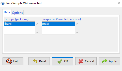
This test in Rcmdr requires that data are in a stacked worksheet and not in unstacked worksheet with two columns. If you need help with worksheet format, then see Part07 in Mike’s Workbook for Biostatistics.

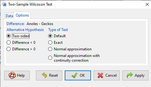
We choose from the Rcmdr Nonparametric statistics menu the Two-sample Wilcoxon test (Fig. \(\PageIndex{3}\)), then a two-tailed test of the null hypothesis (Fig. \(\PageIndex{4}\)) and elect to use the defaults for the tests and calculations of P-values.

Figure \(\PageIndex{3}\): Screenshot Rcmdr menu 2 sample Wilcoxon test. Options are selected by clicking on “Options” tab (see Fig. \(\PageIndex{4}\))

Figure \(\PageIndex{4}\): Screenshot of options tab Rcmdr menu 2 sample Wilcoxon test. Keep defaults to run the “Wilcoxon test.”

Don’t forget to stack the data. Rcmdr won’t produce an error message if the data set is in the unstacked, improper conformation. Instead, Rcmdr menu options will not be available. For example, Fig. \(\PageIndex{5}\) shows a Two-sample Wilcoxon test… dimmed from view, not available for selection.

Figure \(\PageIndex{5}\): Screenshot of Rcmdr menu. Note Two-sample Wilcoxon test… is not available.

The results of the test, copied from the Output window, are shown below.

wilcox.test(Mass ~ Lizard, alternative="two.sided", data=LizardStacked)

Wilcoxon rank sum test
data: Mass by Lizard
W = 14, p-value = 0.1143
alternative hypothesis: true location shift is not equal to 0

The calculation of the Wilcoxon test statistic (W) is straightforward, involving summing the ranks. Obtaining the p-value of the test of the null is a bit more involved as it depends on permutations of all possible combinations of differences. For us, R will do nicely with the details, and we just need to check the p-value.

Here, we see that the medians are 5.6 g for the Anolis, and 2.8 g for the geckos. The associated p-value is 0.1143. Thus, we fail to reject the null hypothesis and conclude that there was no difference in median body mass. Note that this is the same general conclusion we got when we ran a independent \(t\)-test on this data set: there is no difference between day one and day two.

---

Questions

1. Conduct an independent \(t\)-test on the Lizard body mass data.
   • Make a box plot to display the two groups and describe the middle and variability.
   • Compare results of test of hypothesis. do they agree with the Wilcoxon test? If not, list possible reasons why the two tests disagree.
2. Using the dataset below, test null hypothesis using independent \(t\)-test, Welch’s test, and nonparametric Wilcoxon’s test.
   • Make a box plot to display the two groups and describe the middle and variability.
   • Compare results of test of hypothesis. do they agree with the Wilcoxon test? If not, list possible reasons why the tests disagree.

Data set

var1	var2
5.84	5.93
5.72	5.95
5.75	6.02
5.78	5.81
5.81	6.16
5.81	5.95
5.73	6.09
5.77	5.89
5.76	5.99
5.86	5.60
5.84	6.16
5.83	6.16
5.80	6.06
5.78	6.07
5.89	5.66
5.83	6.14
5.79	5.99
5.84	6.15
5.90	5.81
5.86	6.20