Normal Random Variables

CO-6: Apply basic concepts of probability, random variation, and commonly used statistical probability distributions.

Learning Objectives

LO 6.2: Apply the standard deviation rule to the special case of distributions having the “normal” shape.

Video

Video: Normal Random Variables (2:08)

In the Exploratory Data Analysis unit of this course, we encountered data sets, such as lengths of human pregnancies, whose distributions naturally followed a symmetric unimodal bell shape, bulging in the middle and tapering off at the ends.

Many variables, such as pregnancy lengths, shoe sizes, foot lengths, and other human physical characteristics exhibit these properties: symmetry indicates that the variable is just as likely to take a value a certain distance below its mean as it is to take a value that same distance above its mean; the bell-shape indicates that values closer to the mean are more likely, and it becomes increasingly unlikely to take values far from the mean in either direction.

The particular shape exhibited by these variables has been studied since the early part of the nineteenth century, when they were first called “normal” as a way of suggesting their depiction of a common, natural pattern.

Observations of Normal Distributions

There are many normal distributions. Even though all of them have the bell-shape, they vary in their center and spread.

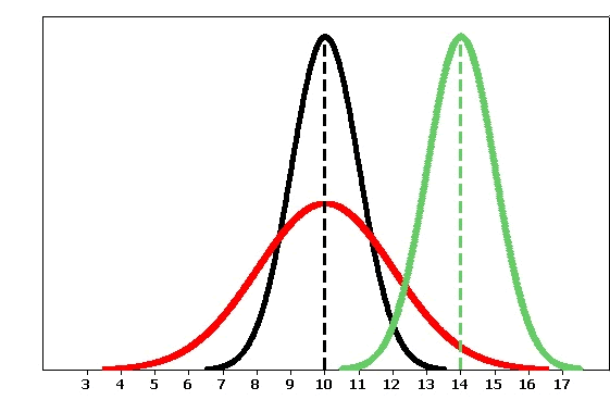
More specifically, the shape of the distribution is determined by its mean (mu, μ) and the spread is determined by its standard deviation (sigma, σ).

Some observations we can make as we look at this graph are:

• The black and the red normal curves have means or centers at μ = mu = 10. However, the red curve is more spread out and thus has a larger standard deviation. As you look at these two normal curves, notice that as the red graph is squished down, the spread gets larger, thus allowing the area under the curve to remain the same.
• The black and the green normal curves have the same standard deviation or spread (the range of the black curve is 6.5-13.5, and the green curve’s range is 10.5-17.5).

Even more important than the fact that many variables themselves follow the normal curve is the role played by the normal curve in sampling theory, as we’ll see in the next section in our unit on probability.

Understanding the normal distribution is an important step in the direction of our overall goal, which is to relate sample means or proportions to population means or proportions. The goal of this section is to better understand normal random variables and their distributions.

The Standard Deviation Rule for Normal Random Variables

We began to get a feel for normal distributions in the Exploratory Data Analysis (EDA) section, when we introduced the Standard Deviation Rule (or the 68-95-99.7 rule) for how values in a normally-shaped sample data set behave relative to their sample mean (x-bar) and sample standard deviation (s).

This is the same rule that dictates how the distribution of a normal random variable behaves relative to its mean (mu, μ) and standard deviation (sigma, σ). Now we use probability language and notation to describe the random variable’s behavior.

For example, in the EDA section, we would have said “68% of pregnancies in our data set fall within 1 standard deviation (s) of their mean (x-bar).” The analogous statement now would be “If X, the length of a randomly chosen pregnancy, is normal with mean (mu, μ) and standard deviation (sigma, σ), then

\(0.68 = P(\mu - \sigma < X < \mu + \sigma)\)

In general, if X is a normal random variable, then the probability is

• 68% that X falls within 1 standard deviation (sigma, σ) of the mean (mu, μ)
• 95% that X falls within 2 standard deviations (sigma, σ) of the mean (mu, μ)
• 99.7% that X falls within 3 standard deviation (sigma, σ) of the mean (mu, μ).

Using probability notation, we may write

\begin{aligned}
&0.68=P(\mu-\sigma<X<\mu+\sigma) \\
&0.95=P(\mu-2 \sigma<X<\mu+2 \sigma) \\
&0.997=P(\mu-3 \sigma<X<\mu+3 \sigma)
\end{aligned}

Comment

• Notice that the information from the rule can be interpreted from the perspective of the tails of the normal curve:
  • Since 0.68 is the probability of being within 1 standard deviation of the mean, (1 – 0.68) / 2 = 0.16 is the probability of being further than 1 standard deviation below the mean (or further than 1 standard deviation above the mean.)
  • Likewise, (1 – 0.95) / 2 = 0.025 is the probability of being more than 2 standard deviations below (or above) the mean.
  • And (1 – 0.997) / 2 = 0.0015 is the probability of being more than 3 standard deviations below (or above) the mean.
• The three figures below illustrate this.

EXAMPLE: Foot Length

Suppose that foot length of a randomly chosen adult male is a normal random variable with mean μ = mu = 11 and standard deviation σ = sigma =1.5. Then the Standard Deviation Rule lets us sketch the probability distribution of X as follows:

(a) What is the probability that a randomly chosen adult male will have a foot length between 8 and 14 inches?

0.95, or 95%.

(b) An adult male is almost guaranteed (.997 probability) to have a foot length between what two values?

6.5 and 15.5 inches.

(c) The probability is only 2.5% that an adult male will have a foot length greater than how many inches?

14. (See image below)

Now you should try a few. (Use the figure that is just before part (a) to help you.)

Learn by Doing: Using the Standard Deviation Rule

Comment

• Notice that there are two types of problems we may want to solve: those like (a), (d) and (e), in which a particular interval of values of a normal random variable is given, and we are asked to find a probability, and those like (b), (c) and (f), in which a probability is given and we are asked to identify what the normal random variable’s values would be.

Did I Get This?: Using the Standard Deviation Rule

Learn by Doing: Normal Random Variables

Let’s go back to our example of foot length:

EXAMPLE: Foot Length

How likely or unlikely is it for a male’s foot length to be more than 13 inches?

Since 13 inches doesn’t happen to be exactly 1, 2, or 3 standard deviations away from the mean, we would only be able to give a very rough estimate of the probability at this point.

Clearly, the Standard Deviation Rule only describes the tip of the iceberg, and while it serves well as an introduction to the normal curve, and gives us a good sense of what would be considered likely and unlikely values, it is very limited in the probability questions it can help us answer.

Here is another familiar normal distribution:

EXAMPLE: SAT Scores

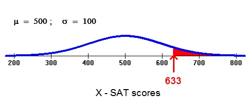
Suppose we are interested in knowing the probability that a randomly selected student will score 633 or more on the math portion of his or her SAT (this is represented by the red area). Again, 633 does not fall exactly 1, 2, or 3 standard deviations above the mean.

Notice, however, that an SAT score of 633 and a foot length of 13 are both about 1/3 of the way between 1 and 2 standard deviations. As you continue to read, you’ll realize that this positioning relative to the mean is the key to finding probabilities.

Standard Normal Distribution

CO-6: Apply basic concepts of probability, random variation, and commonly used statistical probability distributions.

Video

Video: Standard Normal Distribution (4:12)

Finding Probabilities for a Normal Random Variable

Learning Objectives

LO 6.17: Find probabilities associated with a specified normal distribution.

As we saw, the Standard Deviation Rule is very limited in helping us answer probability questions, and basically limited to questions involving values that fall exactly 1, 2, and 3 standard deviations away from the mean. How do we answer probability questions in general? The key is the position of the value relative to the mean, measured in standard deviations.

We can approach the answering of probability questions two possible ways: a table and technology. In the next sections, you will learn how to use the “standard normal table,” and then how the same calculations can be done with technology.

Standardizing Values

The first step to assessing a probability associated with a normal value is to determine the relative value with respect to all the other values taken by that normal variable. This is accomplished by determining how many standard deviations below or above the mean that value is.

EXAMPLE: Foot Length

How many standard deviations below or above the mean male foot length is 13 inches? Since the mean is 11 inches, 13 inches is 2 inches above the mean.

Since a standard deviation is 1.5 inches, this would be 2 / 1.5 = 1.33 standard deviations above the mean. Combining these two steps, we could write:

(13 in. – 11 in.) / (1.5 inches per standard deviation) = (13 – 11) / 1.5 standard deviations = +1.33 standard deviations.

In the language of statistics, we have just found the z-score for a male foot length of 13 inches to be z = +1.33. Or, to put it another way, we have standardized the value of 13.

In general, the standardized value z tells how many standard deviations below or above the mean the original value is, and is calculated as follows:

z-score = (value – mean)/standard deviation

The convention is to denote a value of our normal random variable X with the letter “x.”

\(z=\dfrac{x-\mu}{\sigma}\)

Notice that since the standard deviation (sigma, σ) is always positive, for values of x above the mean (mu, μ), z will be positive; for values of x below the mean (mu, μ), z will be negative.

Let’s go back to our foot length example, and answer some more questions.

EXAMPLE: Foot Length

(a) What is the standardized value for a male foot length of 8.5 inches? How does this foot length relate to the mean?

z = (8.5 – 11) / 1.5 = -1.67. This foot length is 1.67 standard deviations below the mean.

(b) A man’s standardized foot length is +2.5. What is his actual foot length in inches?

If z = +2.5, then his foot length is 2.5 standard deviations above the mean. Since the mean is 11, and each standard deviation is 1.5, we get that the man’s foot length is: 11 + 2.5(1.5) = 14.75 inches.

---

Note that z-scores also allow us to compare values of different normal random variables. Here is an example:

(c) In general, women’s foot length is shorter than men’s. Assume that women’s foot length follows a normal distribution with a mean of 9.5 inches and standard deviation of 1.2. Ross’ foot length is 13.25 inches, and Candace’s foot length is only 11.6 inches. Which of the two has a longer foot relative to his or her gender group?

To answer this question, let’s find the z-score of each of these two normal values, bearing in mind that each of the values comes from a different normal distribution.

Ross: z-score = (13.25 – 11) / 1.5 = 1.5 (Ross’ foot length is 1.5 standard deviations above the mean foot length for men).

Candace: z-score = (11.6 – 9.5) / 1.2 = 1.75 (Candace’s foot length is 1.75 standard deviations above the mean foot length for women).

Note that even though Ross’ foot is longer than Candace’s, Candace’s foot is longer relative to their respective genders.

Comment:

• Part (c) above illustrates how z-scores become crucial when you want to compare distributions.

Did I Get This?: Standardized Scores (z-scores)

Finding Probabilities with the Normal Calculator and Table

Now that you have learned to assess the relative value of any normal value by standardizing, the next step is to evaluate probabilities. In other contexts, as mentioned before, we will first take the conventional approach of referring to a normal table, which tells the probability of a normal variable taking a value less than any standardized score z.

Standard Normal Table

Since normal curves are symmetric about their mean, it follows that the curve of z scores must be symmetric about 0. Since the total area under any normal curve is 1, it follows that the areas on either side of z = 0 are both 0.5. Also, according to the Standard Deviation Rule, most of the area under the standardized curve falls between z = -3 and z = +3.

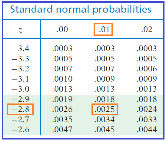
The normal table outlines the precise behavior of the standard normal random variable Z, the number of standard deviations a normal value x is below or above its mean. The normal table provides probabilities that a standardized normal random variable Z would take a value less than or equal to a particular value z*.

These particular values are listed in the form *.* in rows along the left margins of the table, specifying the ones and tenths. The columns fine-tune these values to hundredths, allowing us to look up the probability of being below any standardized value z of the form *.**.

For example, in the part of the table shown below, we can see that for a z-score of -2.81, we would find P(Z < -2.81) = 0.0025.

By construction, the probability P(Z < z*) equals the area under the z curve to the left of that particular value z*.

A quick sketch is often the key to solving normal problems easily and correctly.

Although normal tables are the traditional way to solve these problems, you can also use the normal calculator.

Normal Distribution Calculator: Non-JAVA Version

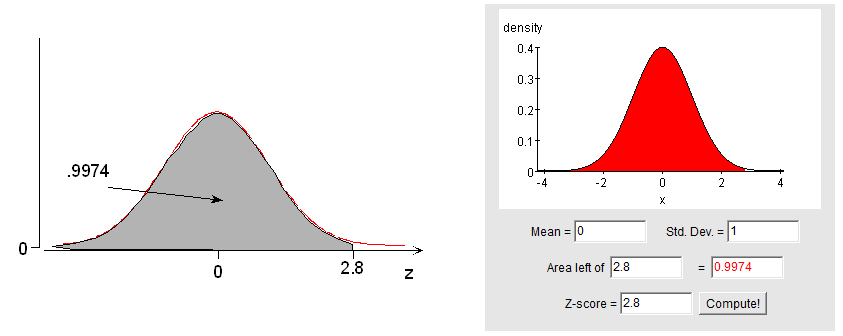
The image below illustrates the results of using the online calculator to find P(Z < -2.81) and P(Z < 1.15). Notice that the calculator behaves exactly as the table.

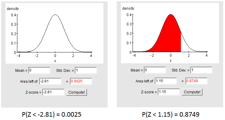
It is your choice to use the table or the online calculator but we will usually illustrate with the online calculator.

EXAMPLE: Standard Normal Probabilities

(a) What is the probability of a normal random variable taking a value less than 2.8 standard deviations above its mean?

P(Z < 2.8) = 0.9974 or 99.74%.

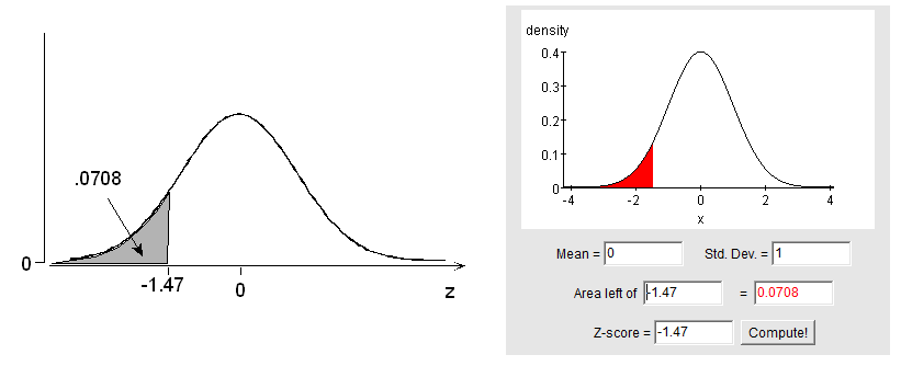
(b) What is the probability of a normal random variable taking a value lower than 1.47 standard deviations below its mean?

P(Z < -1.47) = 0.0708, or 7.08%.

(c) What is the probability of a normal random variable taking a value more than 0.75 standard deviations above its mean?

The fact that the problem involves the word “more” rather than “less” should not be overlooked! Our normal calculator provides left-tail probabilities, and adjustments must be made for any other type of problem.

Method 1:

By symmetry of the z curve centered on 0,

P(Z > +0.75) = P(Z < -0.75) = 0.2266.

Method 2:

Because the total area under the normal curve is 1,

P(Z > +0.75) = 1 – P(Z < +0.75) = 1 – 0.7734 = 0.2266.

[Note: most students prefer to use Method 1, which does not require subtracting 4-digit probabilities from 1.]

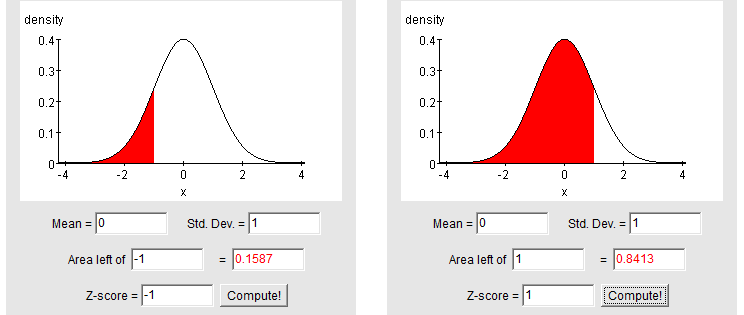
(d) What is the probability of a normal random variable taking a value between 1 standard deviation below and 1 standard deviation above its mean?

To find probabilities in between two standard deviations, we must put them in terms of the probabilities below. A sketch is especially helpful here:

P(-1 < Z < +1) = P(Z < +1) – P(Z < -1) = 0.8413 – 0.1587 = 0.6826.

Here are the normal calculator results which would be needed.

Did I Get This?: Standard Normal Probabilities

Comments:

• So far, we have used the normal calculator or table to find a probability, given the number (z) of standard deviations below or above the mean. The solution process when using the table involved first locating the given z value of the form *.** in the margins, then finding the corresponding probability of the form 0.**** inside the table as our answer.

• Now, in Example 2, a probability will be given and we will be asked to find a z value. The solution process using the table involves first locating the given probability of the form 0.**** inside the table, then finding the corresponding z value of the form *.** as our answer. For the online calculator, the solution is as simply typing in the correct probability and having the calculator solve, in reverse, for the z-score.

Finding Standard Normal Scores

Learning Objectives

LO 6.18: Given a probability, find scores associated with a specified normal distribution.

It is often good to think about this process as the reverse of finding probabilities. In these problems, we will be given some information about the area in a range and asked to provide the z-score(s) associated with that range. Common types of questions are

• Find the standard normal z-score corresponding to the top (or bottom) 8%.
• Find the standard normal z-score associated with the 25th percentile.
• Find the standard normal z-scores which contain the middle 40%.

EXAMPLE: Given Probabilities - Find Z-Scores

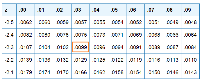
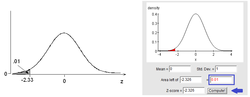
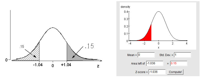
(a) What standard normal z-score is associated with the bottom (or lowest) 1%? The probability is 0.01 that a standardized normal variable takes a value below what particular value of z?

The closest we can come to a probability of 0.01 inside the table is 0.0099, in the z = -2.3 row and 0.03 column: z = -2.33. In other words, the probability is 0.01 that the value of a normal variable is lower than 2.33 standard deviations below its mean.

Using the online calculator, we simply use the calculator in reverse by typing in 0.01 in the “area” box (outlined in blue) and then click “compute” to see the associated z-score. Remember that, like the table, we always need to provide this calculator with the area to the left of the z-score we are currently trying to find.

(b) What standard normal z-score corresponds to the top (or upper) 15%? The probability is 0.15 that a standardized normal variable takes a value above what particular value of z?

Remember that the calculator and table only provide probabilities of being below a certain value, not above. Once again, we must rely on one of the properties of the normal curve to make an adjustment.

Method 1: According to the table, 0.15 (actually 0.1492) is the probability of being below -1.04. By symmetry, 0.15 must also be the probability of being above +1.04. Using the calculator, we can enter 0.15 exactly and find that the corresponding z-score is actually -1.036 giving a final answer of z = +1.036 or +1.04 if we round to two decimal places which is our preference (this results in no differences for students who use the table or the online calculator).

Method 2: If 0.15 is the probability of being above the value we seek, then 1 – 0.15 = 0.85 must be the probability of being below the value we seek. According to the table, 0.85 (actually 0.8508) is the probability of being below +1.04.

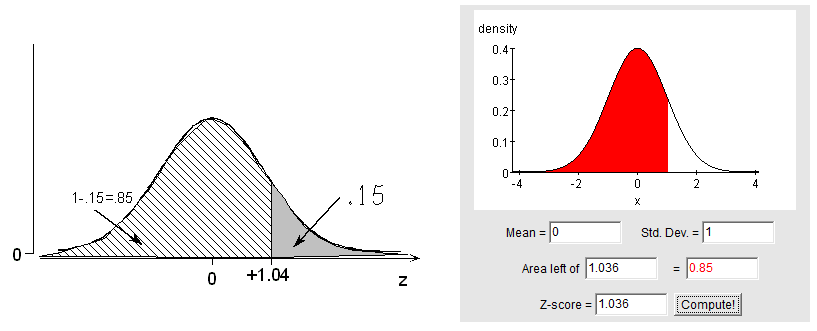
In other words, we have found 0.15 to be the probability that a normal variable takes a value more than 1.04 standard deviations above its mean.

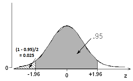
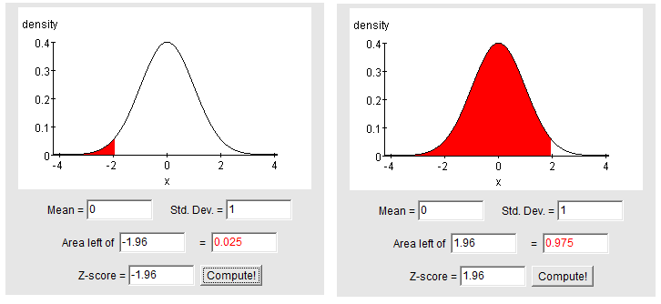
(c) What standard normal z-scores contain the middle 95%? The probability is 0.95 that a normal variable takes a value within how many standard deviations of its mean?

A symmetric area of 0.95 centered at 0 extends to values -z* and +z* such that the remaining (1 – 0.95) / 2 = 0.025 is below -z* and also 0.025 above +z*. The probability is 0.025 that a standardized normal variable is below -1.96. Thus, the probability is 0.95 that a normal variable takes a value within 1.96 standard deviations of its mean. Once again, the Standard Deviation Rule is shown to be just roughly accurate, since it states that the probability is 0.95 that a normal variable takes a value within 2 standard deviations of its mean.

Did I Get This?: Finding Standard Normal Scores

Although the online calculator can provide results for any probability or z-score, our standard normal table, like most, only provides probabilities for z values between -3.49 and +3.49. The following example demonstrates how to handle cases where z exceeds 3.49 in absolute value.

EXAMPLE: Extreme Probabilities

(a) What is the probability of a normal variable being lower than 5.2 standard deviations below its mean?

There is no need to panic about going “off the edge” of the normal table. We already know from the Standard Deviation Rule that the probability is only about (1 -0 .997) / 2 = 0.0015 that a normal value would be more than 3 standard deviations away from its mean in one direction or the other. The table provides information for z values as extreme as plus or minus 3.49: the probability is only 0.0002 that a normal variable would be lower than 3.49 standard deviations below its mean. Any more standard deviations than that, and we generally say the probability is approximately zero.

In this case, we would say the probability of being lower than 5.2 standard deviations below the mean is approximately zero:

P(Z < -5.2) = 0 (approx.)

(b) What is the probability of the value of a normal variable being higher than 6 standard deviations below its mean?

Since the probability of being lower than 6 standard deviations below the mean is approximately zero, the probability of being higher than 6 standard deviations below the mean must be approximately 1.

P(Z > -6) = 1 (approx.)

(c) What is the probability of a normal variable being less than 8 standard deviations above the mean?

Approximately 1. P(Z < +8) = 1 (approx.)

(d) What is the probability of a normal variable being greater than 3.5 standard deviations above the mean?

Approximately 0. P(Z > +3.5) = 0 (approx.)

Normal Applications

CO-6: Apply basic concepts of probability, random variation, and commonly used statistical probability distributions.

Video

Video: Normal Applications (9:41)

Working with Non-standard Normal Values

Learning Objectives

LO 6.17: Find probabilities associated with a specified normal distribution.

In a much earlier example, we wondered,

“How likely or unlikely is a male foot length of more than 13 inches?” We were unable to solve the problem, because 13 inches didn’t happen to be one of the values featured in the Standard Deviation Rule.

Subsequently, we learned how to standardize a normal value (tell how many standard deviations below or above the mean it is) and how to use the normal calculator or table to find the probability of falling in an interval a certain number of standard deviations below or above the mean.

By combining these two skills, we will now be able to answer questions like the one above.

To convert between a non-standard normal (X) and the standard normal (Z) use the following equations, as needed:

\(Z = \dfrac{x - \mu}{\sigma} \quad \quad X = \mu +zQ\)

EXAMPLE: Male Foot Length

Male foot lengths have a normal distribution, with mean (mu, μ) = 11 inches, and standard deviation (sigma, σ) = 1.5 inches.

(a) What is the probability of a foot length of more than 13 inches?

First, we standardize:

\(z = \dfrac{x-\mu}{\sigma} = \dfrac{13-11}{1.5} = +1.33\)

The probability that we seek, P(X > 13), is the same as the probability that a normal variable takes a value greater than 1.33 standard deviations above its mean, i.e. P(Z > +1.33)

This can be solved with the normal calculator or table, after applying the property of symmetry:

P(Z > +1.33) = P(Z < -1.33) = 0.0918.

A male foot length of more than 13 inches is on the long side, but not too unusual: its probability is about 9%.

We can streamline the solution in terms of probability notation and write:

P(X > 13) = P(Z > 1.33) = P(Z < −1.33) = 0.0918

(b) What is the probability of a male foot length between 10 and 12 inches?

The standardized values of 10 and 12 are, respectively,

\(\dfrac{10-11}{1.5} = -0.67\) and \(\dfrac{12-11}{1.5} = 0.67\)

Note: The two z-scores in a “between” problem will not always be the same value. You must calculate both or, in this case, you could recognize that both values are the same distance from the mean and hence result in z-scores which are equal but of opposite signs.

P(-0.67 < Z < +0.67) = P(Z < +0.67) – P(Z < -0.67) = 0.7486 – 0.2514 = 0.4972.

Or, if you prefer the streamlined notation,

P(10 < X < 12) = P(−0.67 < Z < +0.67) = P( Z < +0.67) − P(Z < −0.67) = 0.7486 − 0.2514 = 0.4972.

Comments:

By solving the above example, we inadvertently discovered the quartiles of a normal distribution! P(Z < -0.67) = 0.2514 tells us that roughly 25%, or one quarter, of a normal variable’s values are less than 0.67 standard deviations below the mean.

P(Z < +0.67) = 0.7486 tells us that roughly 75%, or three quarters, are less than 0.67 standard deviations above the mean.

And of course the median is equal to the mean, since the distribution is symmetric, the median is 0 standard deviations away from the mean.

Be sure to verify these results for yourself using the calculator or table!

Let’s look at another example.

EXAMPLE: Length of a Human Pregnancy

Length (in days) of a randomly chosen human pregnancy is a normal random variable with mean (mu, μ) = 266 and standard deviation (sigma, σ) = 16.

(a) Find Q1, the median, and Q3. Using the z-scores we found in the previous example we have

Q1 = 266 – 0.67(16) = 255

median = mean = 266

Q3 = 266 + 0.67(16) = 277

Thus, the probability is 1/4 that a pregnancy will last less than 255 days; 1/2 that it will last less than 266 days; 3/4 that it will last less than 277 days.

(b) What is the probability that a randomly chosen pregnancy will last less than 246 days?

Since (246 – 266) / 16 = -1.25, we write

P(X < 246) = P(Z < −1.25) = 0.1056

(c) What is the probability that a randomly chosen pregnancy will last longer than 240 days?

Since (240 – 266) / 16 = -1.63, we write

P(X > 240) = P(Z > −1.63) = P(Z < +1.63) = 0.9484

Since the mean is 266 and the standard deviation is 16, most pregnancies last longer than 240 days.

(d) What is the probability that a randomly chosen pregnancy will last longer than 500 days?

Method 1:

Common sense tells us that this would be impossible.

Method 2:

The standardized value of 500 is (500 – 266) / 16 = +14.625.

P(X > 500) = P(Z > 14.625) = 0.

(e) Suppose a pregnant woman’s husband has scheduled his business trips so that he will be in town between the 235th and 295th days. What is the probability that the birth will take place during that time?

The standardized values are (235 – 266) / 16) = -1.94 and (295 – 266) / 16 = +1.81.

P(235 < X < 295) = P(−1.94 < Z < +1.81) = P(Z < +1.81) − P(Z < −1.94) = 0.9649 − 0.0262 = 0.9387.

There is close to a 94% chance that the husband will be in town for the birth.

Be sure to verify these results for yourself using the calculator or table!

The purpose of the next activity is to give you guided practice at solving word problems that involve normal random variables. In particular, we’ll solve problems like the examples you just went over, in which you are asked to find the probability that a normal random variable falls within a certain interval.

Learn by Doing: Find Normal Probabilities

The previous examples most followed the same general form: given values of a normal random variable, you were asked to find an associated probability. The two basic steps in the solution process were to

• Standardize to Z;

• Find associated probabilities using the standard normal calculator or table.

Finding Normal Scores

Learning Objectives

LO 6.18: Given a probability, find scores associated with a specified normal distribution.

The next example will be a different type of problem: given a certain probability, you will be asked to find the associated value of the normal random variable. The solution process will go more or less in reverse order from what it was in the previous examples.

EXAMPLE: Foot Length

Again, foot length of a randomly chosen adult male is a normal random variable with a mean of 11 and standard deviation of 1.5.

(a) The probability is 0.04 that a randomly chosen adult male foot length will be less than how many inches?

According to the normal calculator or table, a probability of 0.04 below (actually 0.0401) is associated with z = -1.75.

In other words, the probability is 0.04 that a normal variable takes a value lower than 1.75 standard deviations below its mean.

For adult male foot lengths, this would be 11 – 1.75(1.5) = 8.375. The probability is 0.04 that an adult male foot length would be less than 8.375 inches.

(b) The probability is 0.10 that an adult male foot will be longer than how many inches? Caution is needed here because of the word “longer.”

Once again, we must remind ourselves that the calculator and table only show the probability of a normal variable taking a value lower than a certain number of standard deviations below or above its mean. Adjustments must be made for problems that involve probabilities besides “lower than” or “less than.” As usual, we have a choice of invoking either symmetry or the fact that the total area under the normal curve is 1. Students should examine both methods and decide which they prefer to use for their own purposes.

Method 1:

According to the calculator or table, a probability of 0.10 below is associated with a z value of -1.28. By symmetry, it follows that a probability of 0.10 above has z = +1.28.

We seek the foot length that is 1.28 standard deviations above its mean: 11 + 1.28(1.5) = 12.92, or just under 13 inches.

Method 2: If the probability is 0.10 that a foot will be longer than the value we seek, then the probability is 0.90 that a foot will be shorter than that same value, since the probabilities must sum to 1.

According to the calculator or table, a probability of 0.90 below is associated with a z value of +1.28. Again, we seek the foot length that is 1.28 standard deviations above its mean, or 12.92 inches.

Comment:

• Part (a) in the above example could have been re-phrased as: “0.04 is the proportion of all adult male foot lengths that are below what value?”, which takes the perspective of thinking about the probability as a proportion of occurrences in the long-run. As originally stated, it focuses on the chance of a randomly chosen individual having a normal value in a given interval.

EXAMPLE: Money Spent for Lunch

A study reported that the amount of money spent each week for lunch by a worker in a particular city is a normal random variable with a mean of $35 and a standard deviation of $5.

(a) The probability is 0.97 that a worker will spend less than how much money in a week on lunch?

The z associated with a probability of 0.9700 below is +1.88. The amount that is 1.88 standard deviations above the mean is 35 + 1.88(5) = 44.4, or $44.40.

(b) There is a 30% chance of spending more than how much for lunches in a week?

The z associated with a probability of 0.30 above is +0.52. The amount is 35 + 0.52(5) = 37.6, or $37.60.

Comment:

• Another way of expressing Example (part a.) above would be to ask, “What is the 97th percentile for the amount (X) spent by workers in a week for their lunch?” Many normal variables, such as heights, weights, or exam scores, are often expressed in terms of percentiles.

EXAMPLE:

The height X (in inches) of a randomly chosen woman is a normal random variable with a mean of 65 and a standard deviation of 2.5.

What is the height of a woman who is in the 80th percentile?

A probability of 0.7995 in the table corresponds to z = +0.84. Her height is 65 + 0.84(2.5) = 67.1 inches.

By now we have had practice in solving normal probability problems in both directions: those where a normal value is given and we are asked to report a probability and those where a probability is given and we are asked to report a normal value. Strategies for solving such problems are outlined below:

• Given a normal value x, solve for probability:
  • Standardize: calculate

\(Z = \dfrac{x-\mu}{\sigma}\)

• • If you are using the online calculator: Type the z-score for which you wish to find the area to the left and hit “compute.”
  • If you are using the table: Locate z in the margins of the normal table (ones and tenths for the row, hundredths for the column). Find the corresponding probability (given to four decimal places) of a normal random variable taking a value below z inside the table.
  • (Adjust if the problem involves something other than a “less-than” probability, by invoking either symmetry or the fact that the total area under the normal curve is 1.)

• Given a probability, solve for normal value x:
  • (Adjust if the problem involves something other than a “less-than” probability, by invoking either symmetry or the fact that the total area under the normal curve is 1.)
  • Locate the probability (given to four decimal places) inside the normal table. Using the table, find the corresponding z value in the margins (row for ones and tenths, column for hundredths). Using the calculator, provide the area to left of the z-score you wish to find and hit “compute.”
  • “Unstandardize”: calculate

\(X = \mu + z\sigma\)

This next activity is a continuation of the previous one, and will give you guided practice in solving word problems involving the normal distribution. In particular, we’ll solve problems like the ones you just solved, in which you are given a probability and you are asked to find the normal value associated with it.

Learn by Doing: Find Normal Scores

Normal Approximation for Binomial

The normal distribution can be used as a reasonable approximation to other distributions under certain circumstances. Here we will illustrate this approximation for the binomial distribution.

We will not do any calculations here as we simply wish to illustrate the concept. In the next section on sampling distributions, we will look at another measure related to the binomial distribution, the sample proportion, and at that time we will discuss the underlying normal distribution.

Consider the binomial probability distribution displayed below for n = 20 and p = 0.5.

Now we overlay a normal distribution with the same mean and standard deviation.

And in the final image, we can see the regions for the exact and approximate probabilities shaded.

Unfortunately, the approximated probability, 0.1867, is quite a bit different from the actual probability, 0.2517. However, this example constitutes something of a “worst-case scenario” according to the usual criteria for use of a normal approximation.

Rule of Thumb

Probabilities for a binomial random variable X with n and p may be approximated by those for a normal random variable having the same mean and standard deviation as long as the sample size n is large enough relative to the proportions of successes and failures, p and 1 – p. Our Rule of Thumb will be to require that

np ≥ 10 and n(1 − p) ≥ 10

Continuity Correction

It is possible to improve the normal approximation to the binomial by adjusting for the discrepancy that arises when we make the shift from the areas of histogram rectangles to the area under a smooth curve. For example, if we want to find the binomial probability that X is less than or equal to 8, we are including the area of the entire rectangle over 8, which actually extends to 8.5. Our normal approximation only included the area up to 8.