Continuous Random Variables

CO-6: Apply basic concepts of probability, random variation, and commonly used statistical probability distributions.

Video

Video: Continuous Random Variables (3:59)

In the previous section, we discussed discrete random variables: random variables whose possible values are a list of distinct numbers. We talked about their probability distributions, means, and standard deviations.

We are now moving on to discuss continuous random variables: random variables which can take any value in an interval, so that all of their possible values cannot be listed (such as height, weight, temperature, time, etc.)

As it turns out, most of the methods for dealing with continuous random variables require a higher mathematical level than we needed to deal with discrete random variables. For the most part, the calculation of probabilities associated with a continuous random variable, and its mean and standard deviation, requires knowledge of calculus, and is beyond the scope of this course.

What we will do in this part is discuss the idea behind the probability distribution of a continuous random variable, and show how calculations involving such variables become quite complicated very fast!

We’ll then move on to a special class of continuous random variables – normal random variables. Normal random variables are very common, and play a very important role in statistical inference.

We’ll finish this section by presenting an important connection between the binomial random variable (the special discrete random variable that we presented earlier) and the normal random variable (the special continuous random variable that we’ll present here).

The Probability Distribution of a Continuous Random Variable

Learning Objectives

LO 6.16: Explain how a density function is used to find probabilities involving continuous random variables.

In order to shift our focus from discrete to continuous random variables, let us first consider the probability histogram below for the shoe size of adult males. Let X represent these shoe sizes. Thus, X is a discrete random variable, since shoe sizes can only take whole and half number values, nothing in between.

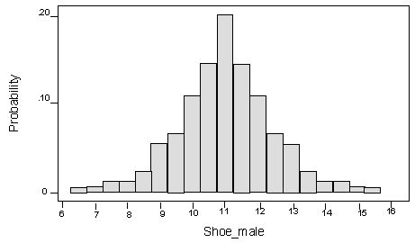
Recall that in all of the previous probability histograms we’ve seen, the X-values were whole numbers. Thus, the width of each bar was 1. The height of each bar was the same as the probability for its corresponding X-value. Due to the principle that states the sum of probabilities of all possible outcomes in the sample space must be 1, the heights of all the rectangles in the histogram must sum to 1. This meant that the area was also 1.

This histogram uses half-sizes. We wish to keep the area = 1, but we still want the horizontal scale to represent half-sizes. Therefore, we must adjust the vertical scale of the histogram. As is, the total area of the histogram rectangles would be .50 times the sum of the probabilities, since the width of each bar is .50. Thus, the area is .50(1) = .50. If we double the vertical scale, the area will double and be 1, just like we want. This means we are changing the vertical scale from “Probability” to “Probability per half size.” The shape and the horizontal scale remain unchanged.

Now we can tell the probability of shoe size taking a value in any interval, just by finding the area of the rectangles over that interval. For instance, the area of the rectangles up to and including 9 shows the probability of having a shoe size less than or equal to 9.

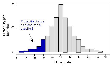
Recall that for a discrete random variable like shoe size, the probability is affected by whether we want strict inequality or not. For example, the area -and corresponding probability – is reduced if we only consider shoe sizes strictly less than 9:

Did I Get This?: Probability for Discrete Random Variables

Transition to Continuous Random Variables

Now we are going to be making the transition from discrete to continuous random variables. Recall that continuous random variables represent measurements and can take on any value within an interval.

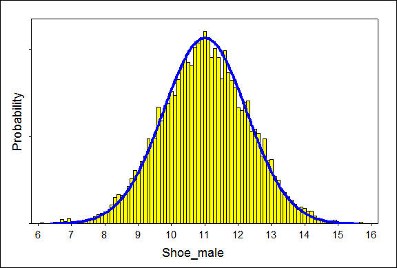
For our shoe size example, this would mean measuring shoe sizes in smaller units, such as tenths, or hundredths. As the number of intervals increases, the width of the bars becomes narrower and narrower, and the graph approaches a smooth curve.

To illustrate this, the following graphs represent two steps in this process of narrowing the widths of the intervals. Specifically, the interval widths are 0.25 and 0.10.

We’ll use these smooth curves to represent the probability distributions of continuous random variables. This idea will be discussed in more detail on the next page.

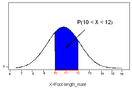
Now consider another random variable X = foot length of adult males. Unlike shoe size, this variable is not limited to distinct, separate values, because foot lengths can take any value over a continuous range of possibilities, so we cannot present this variable with a probability histogram or a table. The probability distribution of foot length (or any other continuous random variable) can be represented by a smooth curve called a probability density curve.

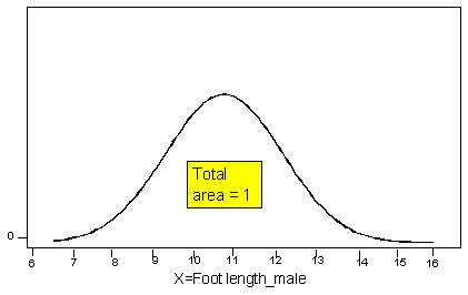
Like the modified probability histogram above, the total area under the density curve equals 1, and the curve represents probabilities by area.

The probability that X gets values in any interval is represented by the area above this interval and below the density curve. In our foot length example, if our interval of interest is between 10 and 12 (marked in red below), and we would like to know P(10 < X < 12), the probability that a randomly chosen male has a foot length anywhere between 10 and 12 inches, we’ll have to find the area above our interval of interest (10,12) and below our density curve, shaded in blue:

If, for example, we are interested in P(X < 9), the probability that a randomly chosen male has a foot length of less than 9 inches, we’ll have to find the area shaded in blue below:

Comments:

• We have seen that for a discrete random variable like shoe size, whether we have a strict inequality or not does matter when solving for probabilities. In contrast, for a continuous random variable like foot length, the probability of a foot length of less than or equal to 9 will be the same as the probability of a foot length of strictly less than 9. In other words, P(X < 9) = P(X ≤ 9).Visually, in terms of our density curve, the area under the curve up to and including a certain point is the same as the area up to and excluding the point, because there is no area over a single point. Conceptually, because a continuous random variable has infinitely many possible values, technically the probability of any single value occurring is zero!

• It should be clear now why the total area under any probability density curve must be 1. The total area under the curve represents P(X gets a value in the interval of its possible values). Clearly, according to the rules of probability this must be 1, or always true.

• Density curves, like probability histograms, may have any shape imaginable as long as the total area underneath the curve is 1.

Let’s Summarize

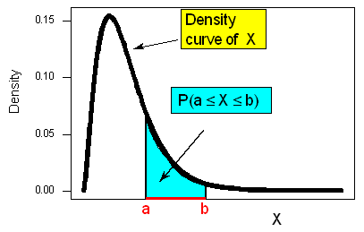
The probability distribution of a continuous random variable is represented by a probability density curve.

The probability that X gets a value in any interval of interest is the area above this interval and below the density curve.

Now that we see how probabilities are found for continuous random variables, we understand why it is more complicated than finding probabilities in the discrete case. As anyone who has studied calculus can attest, finding the area under a curve can be difficult. The general approach is to use integrals. For those of you who did study calculus, the following should be familiar….

where f(x) represents the density curve.

For those who did not study calculus, don’t worry about it. This kind of calculation is definitely beyond the scope of this course.

In this course, we will encounter several important density curves—those for normal random variables, t random variables, chi-square random variables, and F random variables. Normal and t distributions are bell-shaped (single-peaked and symmetric) like the density curve in the foot length example; chi-square and F distributions are single-peaked and skewed right, like in the figure above.

Rather than get bogged down in the calculus of solving for areas under curves, we will find probabilities for the above-mentioned random variables by consulting tables. Also, statistical software automatically provides such probabilities in the appropriate context.

In the next section, we will study in more depth one of those random variables, the normal random variable, and see how we can find probabilities associated with it using software and tables.