Binomial Random Variables

CO-6: Apply basic concepts of probability, random variation, and commonly used statistical probability distributions.

Review:

• Basic Probability Rules
• Conditional Probability and Independence

Video: Binomial Random Variables (12:52)

So far, in our discussion about discrete random variables, we have been introduced to:

1. The probability distribution, which tells us which values a variable takes, and how often it takes them.
2. The mean of the random variable, which tells us the long-run average value that the random variable takes.
3. The standard deviation of the random variable, which tells us a typical (or long-run average) distance between the mean of the random variable and the values it takes.

We will now introduce a special class of discrete random variables that are very common, because as you’ll see, they will come up in many situations – binomial random variables.

Here’s how we’ll present this material.

• First, we’ll explain what kind of random experiments give rise to a binomial random variable, and how the binomial random variable is defined in those types of experiments.
• We’ll then present the probability distribution of the binomial random variable, which will be presented as a formula, and explain why the formula makes sense.
• We’ll conclude our discussion by presenting the mean and standard deviation of the binomial random variable.

As we just mentioned, we’ll start by describing what kind of random experiments give rise to a binomial random variable. We’ll call this type of random experiment a “binomial experiment.”

Binomial Experiment

Learning Objectives

LO 6.14: When appropriate, apply the binomial model to find probabilities.

Binomial experiments are random experiments that consist of a fixed number of repeated trials, like tossing a coin 10 times, randomly choosing 10 people, rolling a die 5 times, etc.

These trials, however, need to be independent in the sense that the outcome in one trial has no effect on the outcome in other trials.

In each of these repeated trials there is one outcome that is of interest to us (we call this outcome “success”), and each of the trials is identical in the sense that the probability that the trial will end in a “success” is the same in each of the trials.

So for example, if our experiment is tossing a coin 10 times, and we are interested in the outcome “heads” (our “success”), then this will be a binomial experiment, since the 10 trials are independent, and the probability of success is 1/2 in each of the 10 trials.

Let’s summarize and give more examples.

The requirements for a random experiment to be a binomial experiment are:

• a fixed number (n) of trials
• each trial must be independent of the others
• each trial has just two possible outcomes, called “success” (the outcome of interest) and “failure“
• there is a constant probability (p) of success for each trial, the complement of which is the probability (1 – p) of failure, sometimes denoted as q = (1 – p)

In binomial random experiments, the number of successes in n trials is random.

It can be as low as 0, if all the trials end up in failure, or as high as n, if all n trials end in success.

The random variable X that represents the number of successes in those n trials is called a binomial random variable, and is determined by the values of n and p. We say, “X is binomial with n = … and p = …”

EXAMPLE: Random Experiments (Binomial or Not?)

Let’s consider a few random experiments.

In each of them, we’ll decide whether the random variable is binomial. If it is, we’ll determine the values for n and p. If it isn’t, we’ll explain why not.

Example A:

A fair coin is flipped 20 times; X represents the number of heads.

X is binomial with n = 20 and p = 0.5.

Example B:

You roll a fair die 50 times; X is the number of times you get a six.

X is binomial with n = 50 and p = 1/6.

Example C:

Roll a fair die repeatedly; X is the number of rolls it takes to get a six.

X is not binomial, because the number of trials is not fixed.

Example D:

Draw 3 cards at random, one after the other, without replacement, from a set of 4 cards consisting of one club, one diamond, one heart, and one spade; X is the number of diamonds selected.

X is not binomial, because the selections are not independent. (The probability (p) of success is not constant, because it is affected by previous selections.)

Example E:

Draw 3 cards at random, one after the other, with replacement, from a set of 4 cards consisting of one club, one diamond, one heart, and one spade; X is the number of diamonds selected. Sampling with replacement ensures independence.

X is binomial with n = 3 and p = 1/4

Example F:

Approximately 1 in every 20 children has a certain disease. Let X be the number of children with the disease out of a random sample of 100 children. Although the children are sampled without replacement, it is assumed that we are sampling from such a vast population that the selections are virtually independent.

X is binomial with n = 100 and p = 1/20 = 0.05.

Example G:

The probability of having blood type B is 0.1. Choose 4 people at random; X is the number with blood type B.

X is binomial with n = 4 and p = 0.1.

Example H:

A student answers 10 quiz questions completely at random; the first five are true/false, the second five are multiple choice, with four options each. X represents the number of correct answers.

X is not binomial, because p changes from 1/2 to 1/4.

Comments:

• Example D above was not binomial because sampling without replacement resulted in dependent selections.
  • In particular, the probability of the second card being a diamond is very dependent on whether or not the first card was a diamond:
  • the probability is 0 if the first card was a diamond, 1/3 if the first card was not a diamond.

• In contrast, Example E was binomial because sampling with replacement resulted in independent selections:
  • the probability of any of the 3 cards being a diamond is 1/4 no matter what the previous selections have been.

• On the other hand, when you take a relatively small random sample of subjects from a large population, even though the sampling is without replacement, we can assume independence because the mathematical effect of removing one individual from a very large population on the next selection is negligible.
  • For example, in Example F, we sampled 100 children out of the population of all children.
  • Even though we sampled the children without replacement, whether one child has the disease or not really has no effect on whether another child has the disease or not.
  • The same is true for Example (G.).

Did I Get This?: Binomial or Not?

Binomial Probability Distribution – Using Probability Rules

Now that we understand what a binomial random variable is, and when it arises, it’s time to discuss its probability distribution. We’ll start with a simple example and then generalize to a formula.

EXAMPLE: Deck of Cards

Consider a regular deck of 52 cards, in which there are 13 cards of each suit: hearts, diamonds, clubs and spades. We select 3 cards at random with replacement. Let X be the number of diamond cards we got (out of the 3).

We have 3 trials here, and they are independent (since the selection is with replacement). The outcome of each trial can be either success (diamond) or failure (not diamond), and the probability of success is 1/4 in each of the trials.

X, then, is binomial with n = 3 and p = 1/4.

Let’s build the probability distribution of X as we did in the chapter on probability distributions. Recall that we begin with a table in which we:

• record all possible outcomes in 3 selections, where each selection may result in success (a diamond, D) or failure (a non-diamond, N).
• find the value of X that corresponds to each outcome.
• use simple probability principles to find the probability of each outcome.

With the help of the addition principle, we condense the information in this table to construct the actual probability distribution table:

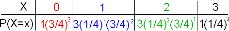
In order to establish a general formula for the probability that a binomial random variable X takes any given value x, we will look for patterns in the above distribution. From the way we constructed this probability distribution, we know that, in general:

Let’s start with the second part, the probability that there will be x successes out of 3, where the probability of success is 1/4.

Notice that the fractions multiplied in each case are for the probability of x successes (where each success has a probability of p = 1/4) and the remaining (3 – x) failures (where each failure has probability of 1 – p = 3/4).

So in general:

Let’s move on to talk about the number of possible outcomes with x successes out of three. Here it is harder to see the pattern, so we’ll give the following mathematical result.

Counting Outcomes

Consider a random experiment that consists of n trials, each one ending up in either success or failure. The number of possible outcomes in the sample space that have exactly k successes out of n is:

\(\left(\begin{array}{l}
n \\
k
\end{array}\right)=\dfrac{n !}{k !(n-k) !}\)

The notation on the left is often read as “n choose k.” Note that n! is read “n factorial” and is defined to be the product 1 * 2 * 3 * … * n. 0! is defined to be 1.

EXAMPLE: Ear Piercings

You choose 12 male college students at random and record whether they have any ear piercings (success) or not. There are many possible outcomes to this experiment (actually, 4,096 of them!).

In how many of the possible outcomes of this experiment are there exactly 8 successes (students who have at least one ear pierced)?

There is no way that we would start listing all these possible outcomes. The result above comes to our rescue.

The result says that in an experiment like this, where you repeat a trial n times (in our case, we repeat it n = 12 times, once for each student we choose), the number of possible outcomes with exactly 8 successes (out of 12) is:

\(\dfrac{12!}{8!(12-8)!} = \dfrac{1*2*3*\cdots*12}{(1*2*3*\cdots*8)(1*2*3*4)} = 495\)

Did I Get This?: Counting Outcomes

EXAMPLE: Card Revisited

Let’s go back to our example, in which we have n = 3 trials (selecting 3 cards). We saw that there were 3 possible outcomes with exactly 2 successes out of 3. The result confirms this since:

\(\dfrac{3!}{2!(3-2)!} = \dfrac{1*2*3}{(1*2)(1)} = \dfrac{6}{2} = 3\)

In general, then

Putting it all together, we get that the probability distribution of X, which is binomial with n = 3 and p = 1/4 i

\(P(X=x)=\dfrac{3 !}{\mathrm{x} !(3-x) !}\left(\dfrac{1}{4}\right)^{x}\left(\dfrac{3}{4}\right)^{3-x} \quad x=0,1,2,3\)

In general, the number of ways to get x successes (and n – x failures) in n trials is

\(\left(\begin{array}{l}
n \\
k
\end{array}\right)=\dfrac{n !}{k !(n-k) !}\)

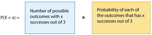
Therefore, the probability of x successes (and n – x failures) in n trials, where the probability of success in each trial is p (and the probability of failure is 1 – p) is equal to the number of outcomes in which there are x successes out of n trials, times the probability of x successes, times the probability of n – x failures:

Binomial Probability Formula for P(X = x)

\(P(X=x)=\dfrac{n !}{x !(n-x) !} p^{x}(1-p)^{(n-x)}\)

where x may take any value 0, 1, … , n.

Let’s look at another example:

EXAMPLE: Blood Type A

The probability of having blood type A is 0.4. Choose 4 people at random and let X be the number with blood type A.

X is a binomial random variable with n = 4 and p = 0.4.

As a review, let’s first find the probability distribution of X the long way: construct an interim table of all possible outcomes in S, the corresponding values of X, and probabilities. Then construct the probability distribution table for X.

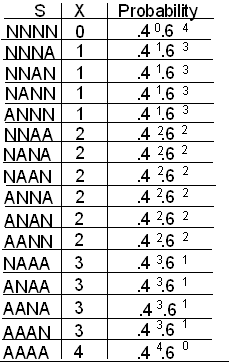
As usual, the addition rule lets us combine probabilities for each possible value of X:

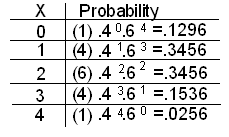
Now let’s apply the formula for the probability distribution of a binomial random variable, and see that by using it, we get exactly what we got the long way.

Recall that the general formula for the probability distribution of a binomial random variable with n trials and probability of success p is:

\(P(X=x)=\dfrac{n !}{x !(n-x) !} p^{x}(1-p)^{(n-x)} \text { for } \mathrm{x}=0,1,2,3, \ldots, \mathrm{n}\)

In our case, X is a binomial random variable with n = 4 and p = 0.4, so its probability distribution is:

\(P(X=x)=\dfrac{4 !}{x !(4-x) !}(0.4)^{x}(0.6)^{4-x} \text { for } \mathrm{x}=0,1,2,3,4\)

Let’s use this formula to find P(X = 2) and see that we get exactly what we got before.

\(P(X=2)=\dfrac{4 !}{2 !(4-2) !}(0.4)^{2}(0.6)^{4-2}=\dfrac{1^{*} 2^{*} 3^{*} 4}{\left(1^{*} 2\right)\left(1^{*} 2\right)}(0.4)^{2}(0.6)^{2}=0.3456\)

Learn by Doing: Binomial Probabilities (Using Online Calculator)

Now let’s look at some truly practical applications of binomial random variables.

EXAMPLE: Airline Flights

Past studies have shown that 90% of the booked passengers actually arrive for a flight. Suppose that a small shuttle plane has 45 seats. We will assume that passengers arrive independently of each other. (This assumption is not really accurate, since not all people travel alone, but we’ll use it for the purposes of our experiment).

Many times airlines “overbook” flights. This means that the airline sells more tickets than there are seats on the plane. This is due to the fact that sometimes passengers don’t show up, and the plane must be flown with empty seats. However, if they do overbook, they run the risk of having more passengers than seats. So, some passengers may be unhappy. They also have the extra expense of putting those passengers on another flight and possibly supplying lodging.

With these risks in mind, the airline decides to sell more than 45 tickets. If they wish to keep the probability of having more than 45 passengers show up to get on the flight to less than 0.05, how many tickets should they sell?

This is a binomial random variable that represents the number of passengers that show up for the flight. It has p = 0.90, and n to be determined.

Suppose the airline sells 50 tickets. Now we have n = 50 and p = 0.90. We want to know P(X > 45), which is 1 – P(X ≤ 45) = 1 – 0.57 or 0.43. Obviously, all the details of this calculation were not shown, since a statistical technology package was used to calculate the answer. This is certainly more than 0.05, so the airline must sell fewer seats.

If we reduce the number of tickets sold, we should be able to reduce this probability. We have calculated the probabilities in the following table:

# tickets sold	P(X > 45)
50	45)" class="lt-stats-31283">45)" class=" ">0.43
49	45)" class="lt-stats-31283">45)" class=" ">0.26
48	45)" class="lt-stats-31283">45)" class=" ">0.13
47	45)" class="lt-stats-31283">45)" class=" ">0.04
46	45)" class="lt-stats-31283">45)" class=" ">0.008

From this table, we can see that by selling 47 tickets, the airline can reduce the probability that it will have more passengers show up than there are seats to less than 5%.

Note: For practice in finding binomial probabilities, you may wish to verify one or more of the results from the table above.

Learn by Doing: Binomial Application

Mean and Standard Deviation of the Binomial Random Variable

Learning Objectives

LO 6.15: Find the mean, variance, and standard deviation of a binomial random variable.

Now that we understand how to find probabilities associated with a random variable X which is binomial, using either its probability distribution formula or software, we are ready to talk about the mean and standard deviation of a binomial random variable. Let’s start with an example:

EXAMPLE: Blood Type B - Mean

Overall, the proportion of people with blood type B is 0.1. In other words, roughly 10% of the population has blood type B.

Suppose we sample 120 people at random. On average, how many would you expect to have blood type B?

The answer, 12, seems obvious; automatically, you’d multiply the number of people, 120, by the probability of blood type B, 0.1.

This suggests the general formula for finding the mean of a binomial random variable:

Claim:

If X is binomial with parameters n and p, then the mean or expected value of X is:

\(\mu_X = np\)

Although the formula for mean is quite intuitive, it is not at all obvious what the variance and standard deviation should be. It turns out that:

Claim:

The ideal gas law is easy to remember and apply in solving problems, as long as you get the proper values aIf X is binomial with parameters n and p, then the variance and standard deviation of X are:

\begin{aligned}
\sigma_{X}^{2} &=n p(1-p) \\
\sigma_{X} &=\sqrt{n p(1-p)}
\end{aligned}

Comments:

• The binomial mean and variance are special cases of our general formulas for the mean and variance of any random variable. Clearly it is much simpler to use the “shortcut” formulas presented above than it would be to calculate the mean and variance or standard deviation from scratch.

• Remember, these “shortcut” formulas only hold in cases where you have a binomial random variable.

EXAMPLE: Blood Type B - Standard Deviation

Suppose we sample 120 people at random. The number with blood type B should be about 12, give or take how many? In other words, what is the standard deviation of the number X who have blood type B?

Since n = 120 and p = 0.1,

\(\sigma_{X}^{2}=120(0.1)(1-0.1)=10.8 ; \quad \sigma_{X}=\sqrt{10.8} \approx 3.3\)

In a random sample of 120 people, we should expect there to be about 12 with blood type B, give or take about 3.3.

Did I Get This?: Binomial Distribution

Before we move on to continuous random variables, let’s investigate the shape of binomial distributions.

Learn by Doing: Shapes of Binomial Distributions