Unit 3A: Probability
- Page ID
- 31262
\( \newcommand{\vecs}[1]{\overset { \scriptstyle \rightharpoonup} {\mathbf{#1}} } \)
\( \newcommand{\vecd}[1]{\overset{-\!-\!\rightharpoonup}{\vphantom{a}\smash {#1}}} \)
\( \newcommand{\dsum}{\displaystyle\sum\limits} \)
\( \newcommand{\dint}{\displaystyle\int\limits} \)
\( \newcommand{\dlim}{\displaystyle\lim\limits} \)
\( \newcommand{\id}{\mathrm{id}}\) \( \newcommand{\Span}{\mathrm{span}}\)
( \newcommand{\kernel}{\mathrm{null}\,}\) \( \newcommand{\range}{\mathrm{range}\,}\)
\( \newcommand{\RealPart}{\mathrm{Re}}\) \( \newcommand{\ImaginaryPart}{\mathrm{Im}}\)
\( \newcommand{\Argument}{\mathrm{Arg}}\) \( \newcommand{\norm}[1]{\| #1 \|}\)
\( \newcommand{\inner}[2]{\langle #1, #2 \rangle}\)
\( \newcommand{\Span}{\mathrm{span}}\)
\( \newcommand{\id}{\mathrm{id}}\)
\( \newcommand{\Span}{\mathrm{span}}\)
\( \newcommand{\kernel}{\mathrm{null}\,}\)
\( \newcommand{\range}{\mathrm{range}\,}\)
\( \newcommand{\RealPart}{\mathrm{Re}}\)
\( \newcommand{\ImaginaryPart}{\mathrm{Im}}\)
\( \newcommand{\Argument}{\mathrm{Arg}}\)
\( \newcommand{\norm}[1]{\| #1 \|}\)
\( \newcommand{\inner}[2]{\langle #1, #2 \rangle}\)
\( \newcommand{\Span}{\mathrm{span}}\) \( \newcommand{\AA}{\unicode[.8,0]{x212B}}\)
\( \newcommand{\vectorA}[1]{\vec{#1}} % arrow\)
\( \newcommand{\vectorAt}[1]{\vec{\text{#1}}} % arrow\)
\( \newcommand{\vectorB}[1]{\overset { \scriptstyle \rightharpoonup} {\mathbf{#1}} } \)
\( \newcommand{\vectorC}[1]{\textbf{#1}} \)
\( \newcommand{\vectorD}[1]{\overrightarrow{#1}} \)
\( \newcommand{\vectorDt}[1]{\overrightarrow{\text{#1}}} \)
\( \newcommand{\vectE}[1]{\overset{-\!-\!\rightharpoonup}{\vphantom{a}\smash{\mathbf {#1}}}} \)
\( \newcommand{\vecs}[1]{\overset { \scriptstyle \rightharpoonup} {\mathbf{#1}} } \)
\(\newcommand{\longvect}{\overrightarrow}\)
\( \newcommand{\vecd}[1]{\overset{-\!-\!\rightharpoonup}{\vphantom{a}\smash {#1}}} \)
\(\newcommand{\avec}{\mathbf a}\) \(\newcommand{\bvec}{\mathbf b}\) \(\newcommand{\cvec}{\mathbf c}\) \(\newcommand{\dvec}{\mathbf d}\) \(\newcommand{\dtil}{\widetilde{\mathbf d}}\) \(\newcommand{\evec}{\mathbf e}\) \(\newcommand{\fvec}{\mathbf f}\) \(\newcommand{\nvec}{\mathbf n}\) \(\newcommand{\pvec}{\mathbf p}\) \(\newcommand{\qvec}{\mathbf q}\) \(\newcommand{\svec}{\mathbf s}\) \(\newcommand{\tvec}{\mathbf t}\) \(\newcommand{\uvec}{\mathbf u}\) \(\newcommand{\vvec}{\mathbf v}\) \(\newcommand{\wvec}{\mathbf w}\) \(\newcommand{\xvec}{\mathbf x}\) \(\newcommand{\yvec}{\mathbf y}\) \(\newcommand{\zvec}{\mathbf z}\) \(\newcommand{\rvec}{\mathbf r}\) \(\newcommand{\mvec}{\mathbf m}\) \(\newcommand{\zerovec}{\mathbf 0}\) \(\newcommand{\onevec}{\mathbf 1}\) \(\newcommand{\real}{\mathbb R}\) \(\newcommand{\twovec}[2]{\left[\begin{array}{r}#1 \\ #2 \end{array}\right]}\) \(\newcommand{\ctwovec}[2]{\left[\begin{array}{c}#1 \\ #2 \end{array}\right]}\) \(\newcommand{\threevec}[3]{\left[\begin{array}{r}#1 \\ #2 \\ #3 \end{array}\right]}\) \(\newcommand{\cthreevec}[3]{\left[\begin{array}{c}#1 \\ #2 \\ #3 \end{array}\right]}\) \(\newcommand{\fourvec}[4]{\left[\begin{array}{r}#1 \\ #2 \\ #3 \\ #4 \end{array}\right]}\) \(\newcommand{\cfourvec}[4]{\left[\begin{array}{c}#1 \\ #2 \\ #3 \\ #4 \end{array}\right]}\) \(\newcommand{\fivevec}[5]{\left[\begin{array}{r}#1 \\ #2 \\ #3 \\ #4 \\ #5 \\ \end{array}\right]}\) \(\newcommand{\cfivevec}[5]{\left[\begin{array}{c}#1 \\ #2 \\ #3 \\ #4 \\ #5 \\ \end{array}\right]}\) \(\newcommand{\mattwo}[4]{\left[\begin{array}{rr}#1 \amp #2 \\ #3 \amp #4 \\ \end{array}\right]}\) \(\newcommand{\laspan}[1]{\text{Span}\{#1\}}\) \(\newcommand{\bcal}{\cal B}\) \(\newcommand{\ccal}{\cal C}\) \(\newcommand{\scal}{\cal S}\) \(\newcommand{\wcal}{\cal W}\) \(\newcommand{\ecal}{\cal E}\) \(\newcommand{\coords}[2]{\left\{#1\right\}_{#2}}\) \(\newcommand{\gray}[1]{\color{gray}{#1}}\) \(\newcommand{\lgray}[1]{\color{lightgray}{#1}}\) \(\newcommand{\rank}{\operatorname{rank}}\) \(\newcommand{\row}{\text{Row}}\) \(\newcommand{\col}{\text{Col}}\) \(\renewcommand{\row}{\text{Row}}\) \(\newcommand{\nul}{\text{Nul}}\) \(\newcommand{\var}{\text{Var}}\) \(\newcommand{\corr}{\text{corr}}\) \(\newcommand{\len}[1]{\left|#1\right|}\) \(\newcommand{\bbar}{\overline{\bvec}}\) \(\newcommand{\bhat}{\widehat{\bvec}}\) \(\newcommand{\bperp}{\bvec^\perp}\) \(\newcommand{\xhat}{\widehat{\xvec}}\) \(\newcommand{\vhat}{\widehat{\vvec}}\) \(\newcommand{\uhat}{\widehat{\uvec}}\) \(\newcommand{\what}{\widehat{\wvec}}\) \(\newcommand{\Sighat}{\widehat{\Sigma}}\) \(\newcommand{\lt}{<}\) \(\newcommand{\gt}{>}\) \(\newcommand{\amp}{&}\) \(\definecolor{fillinmathshade}{gray}{0.9}\)CO-1: Describe the roles biostatistics serves in the discipline of public health.
CO-6: Apply basic concepts of probability, random variation, and commonly used statistical probability distributions.
Video: Unit 3A: Introduction (5:36)
Review of the Big Picture
LO 1.3: Identify and differentiate between the components of the Big Picture of Statistics
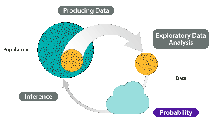
Recall the Big Picture — the four-step process that encompasses statistics (as it is presented in this course):

So far, we’ve discussed the first two steps:
Producing data — how data are obtained, and what considerations affect the data production process.
Exploratory data analysis — tools that help us get a first feel for the data, by exposing their features using visual displays and numerical summaries which help us explore distributions, compare distributions, and investigate relationships.
(Recall that the structure of this course is such that Exploratory Data Analysis was covered first, followed by Producing Data.)
Our eventual goal is Inference — drawing reliable conclusions about the population based on what we’ve discovered in our sample.
In order to really understand how inference works, though, we first need to talk about Probability, because it is the underlying foundation for the methods of statistical inference.
The probability unit starts with an introduction, which will give you some motivating examples and an intuitive and informal perspective on probability.
Why do we need to understand probability?
- We often want to estimate the chance that an event (of interest to us) will occur.
- Many values of interest are probabilities or are derived from probabilities, for example, prevalence rates, incidence rates, and sensitivity/specificity of tests for disease.
- Plus!! Inferential statistics relies on probability to
- Test hypotheses
- Estimate population values, such as the population mean or population proportion.
Probability and Inference
We will use an example to try to explain why probability is so essential to inference.
First, here is the general idea:
As we all know, the way statistics works is that we use a sample to learn about the population from which it was drawn. Ideally, the sample should be random so that it represents the population well.
Recall from the discussion about sampling that when we say that a random sample represents the population well we mean that there is no inherent bias in this sampling technique.
It is important to acknowledge, though, that this does not mean that all random samples are necessarily “perfect.” Random samples are still random, and therefore no random sample will be exactly the same as another.
One random sample may give a fairly accurate representation of the population, while another random sample might be “off,” purely due to chance.
Unfortunately, when looking at a particular sample (which is what happens in practice), we will never know how much it differs from the population.
This uncertainty is where probability comes into the picture. This gives us a way to draw conclusions about the population in the face of the uncertainty that is generated by the use of a random sample.
We use probability to quantify how much we expect random samples to vary.
The following example will illustrate this important point.
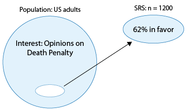
Suppose that we are interested in estimating the percentage of U.S. adults who favor the death penalty.
In order to do so, we choose a random sample of 1,200 U.S. adults and ask their opinion: either in favor of or against the death penalty.
We find that 744 out of the 1,200, or 62%, are in favor. (Comment: although this is only an example, this figure of 62% is quite realistic, given some recent polls).
Here is a picture that illustrates what we have done and found in our example:

Our goal here is inference — to learn and draw conclusions about the opinions of the entire population of U.S. adults regarding the death penalty, based on the opinions of only 1,200 of them.
Can we conclude that 62% of the population favors the death penalty?
- Another random sample could give a very different result. So we are uncertain.
But since our sample is random, we know that our uncertainty is due to chance, and not due to problems with how the sample was collected.
So we can use probability to describe the likelihood that our sample is within a desired level of precision.
For example, probability can answer the question, “How likely is it that our sample estimate is no more than 3% from the true percentage of all U.S. adults who are in favor of the death penalty?”
The answer to this question (which we find using probability) is obviously going to have an important impact on the confidence we can attach to the inference step.
In particular, if we find it quite unlikely that the sample percentage will be very different from the population percentage, then we have a lot of confidence that we can draw conclusions about the population based on the sample.
In the health sciences, a comparable situation to the death penalty example would be when we wish to determine the prevalence of a certain disease or condition.
In epidemiology, the prevalence of a health-related state (typically disease, but also other things like smoking or seat belt use) in a statistical population is defined as the total number of cases in the population, divided by the number of individuals in the population.
As we will see, this is a form of probability.
In practice, we will need to estimate the prevalence using a sample and in order to make inferences about the population from a sample, we will need to understand probability.
The CDC estimates that in 2011, 8.3% of the U.S. population have diabetes. In other words, the CDC estimates the prevalence of diabetes to be 8.3% in the U.S.
There are numerous statistics and graphs reported in this document you should now understand!!
Other common probabilities used in the health sciences are
- (Cumulative) Incidence: the probability that a person with no prior disease will develop disease over some specified time period
- Sensitivity of a diagnostic or screening test: the probability the person tests positive, given the person has the disease. Specificity of a diagnostic or screening test: the probability the person tests negative, given the person does not have the disease. As well as predictive value positive, predictive value negative, false positive rate, false negative rate.
- Survival probability: the probability an individual survives beyond a certain time

